Forecasting diagnostics
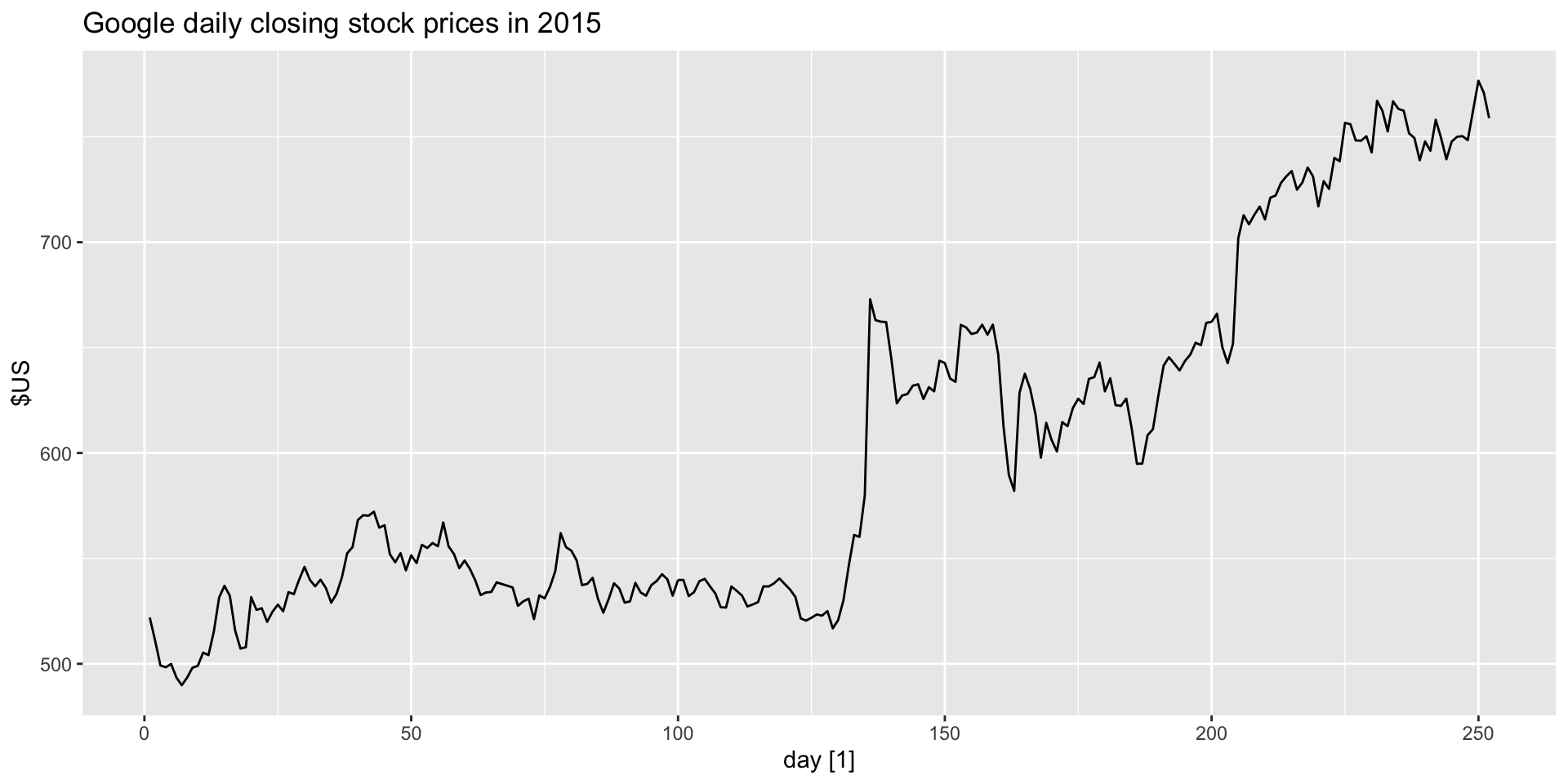
Example: Google closing stock prices
- Innovation residual for a naive forecast?
- \(e_{t} = y_{t} - \hat{y}_{t} = y_{t} - y_{t-1}\).
- And make an autoplot:
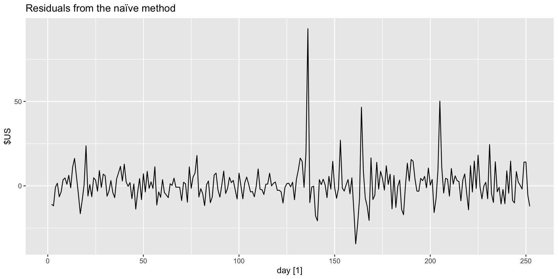
Example: Google closing stock prices residual autoplot
- Autoplot the innovation residuals:
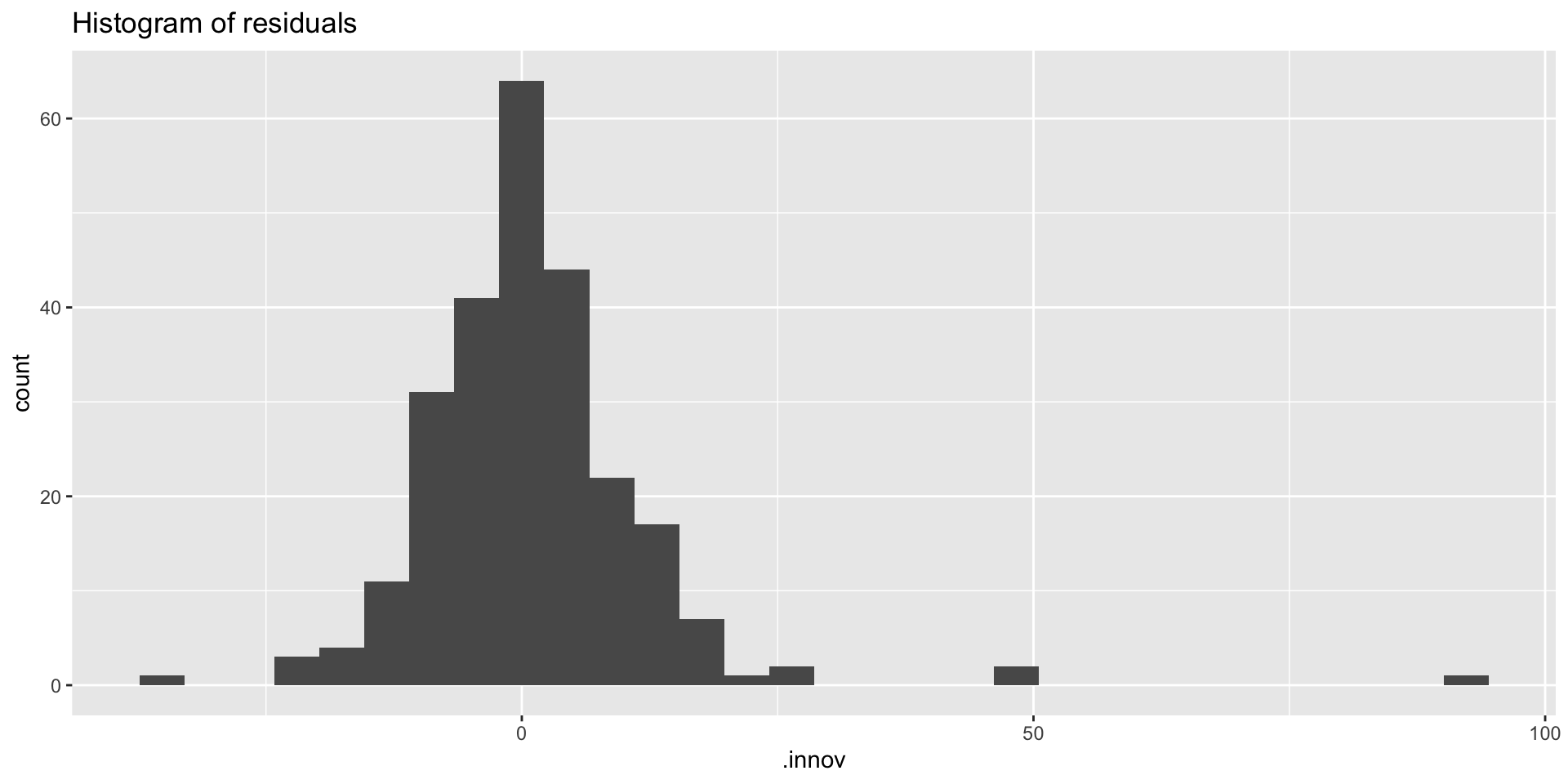
Example: Google closing stock prices residual histogram
-Produce a histogram of the innovation residuals:
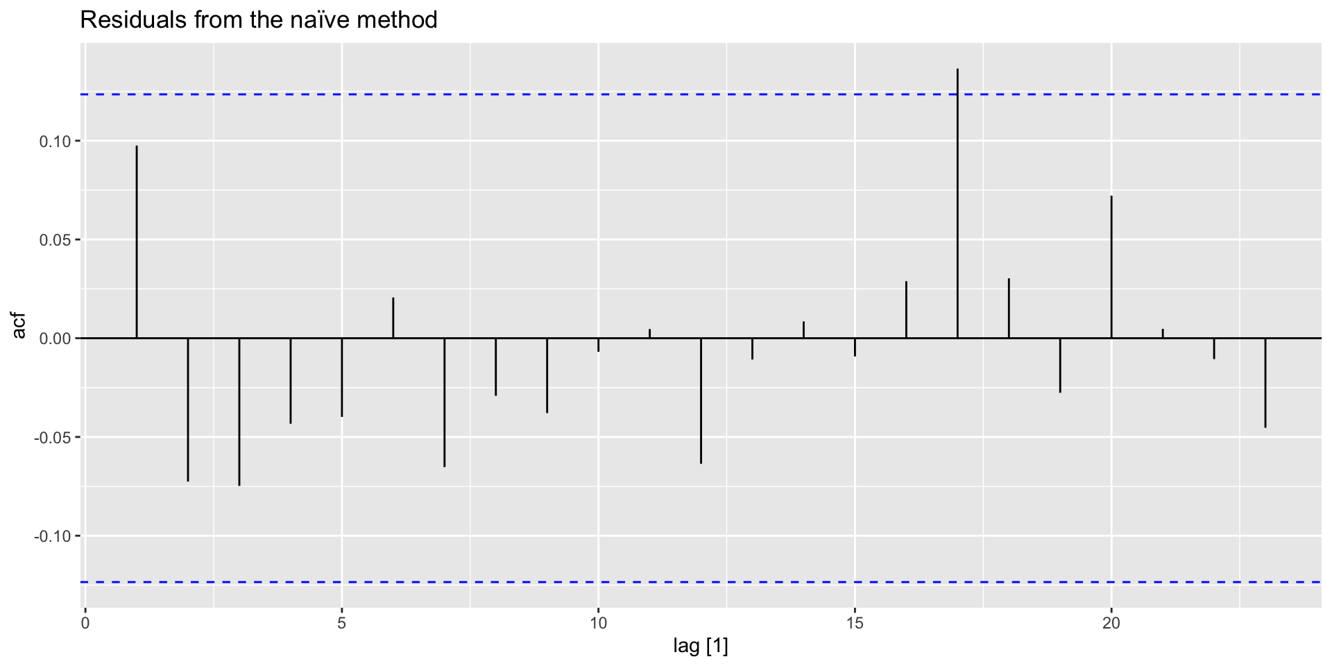
Example: Google closing stock prices ACF plot
- Produce an ACF plot:
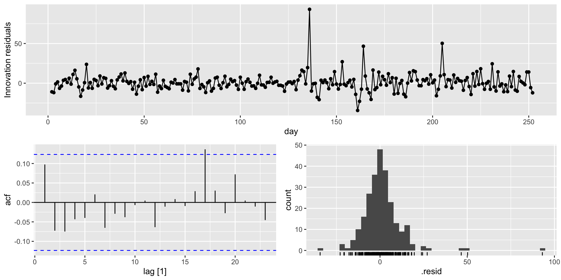
Example: Google closing stock prices tsresiduals()
- You can use
tsresiduals()to produce all of these: