Distributional forecasts and prediction intervals
BUS 323 Forecasting and Risk Analysis
Forecast distributions
- Forecasts have associated probability distribution
- Typically Normal
- Mean: point forecast
Prediction intervals
- 95% interval for a Normally distributed \(h\)-step forecast:
\[ \widehat{y}_{T+h|T} \pm 1.96 \widehat{\sigma}_{h} \]
where \(\widehat{\sigma}_{h}\) is the standard error of the \(h\)-step forecast.
Forecast standard error
- Where do we get \(\widehat{\sigma}_{h}\) from?
- Need residual standard error first
- Next, we can find the distribution standard error.
Forecast standard error: demonstration
- e.g. for a mean forecast:
\[ \widehat{y}_{T+h|T} = \bar{y} \]
The residual is \(e_{T+h} = y_{T+h} - \bar{y}\).
- \(y_{T+h} \sim N(0,\sigma)\).
- \(\bar{y} \sim N(0,\sqrt{\frac{\sigma^{2}}{T}})\).
- Thus \(e_{T+H} \sim N(0, \sqrt{\sigma^{2} + \frac{\sigma^{2}}{T}})\).
Forecast standard error: demonstration
- Constant forecast with this method
\(\rightarrow\) Constant forecast standard error of \(\sigma \sqrt{1 + \frac{1}{t}}\).
Forecast standard errors: other methods
- Mean: \(\widehat{\sigma}_{h} = \widehat{\sigma} \sqrt{1 + \frac{1}{T}}\)
- Naive: \(\widehat{\sigma}_{h} = \widehat{\sigma} \sqrt{h}\)
- Seasonal naive: \(\widehat{\sigma}_{h} = \widehat{\sigma} \sqrt{k+1}\)
- where \(k\) represents \(\frac{h-1}{m}\) and \(m\) represents the seasonal period
- Drift: \(\widehat{\sigma}_{h} = \widehat{\sigma} \sqrt{h(1 + \frac{h}{T-1})}\)
Computing prediction intervals with R
- Using the pakcage
fable(withinfpp3) and functionhilo():
| Symbol | .model | day | Close | .mean | 80% | 95% |
|---|---|---|---|---|---|---|
| GOOG | NAIVE(Close) | 253 | N(759, 125) | 758.88 | [744.5400, 773.2200]80 | [736.9488, 780.8112]95 |
| GOOG | NAIVE(Close) | 254 | N(759, 250) | 758.88 | [738.6001, 779.1599]80 | [727.8646, 789.8954]95 |
| GOOG | NAIVE(Close) | 255 | N(759, 376) | 758.88 | [734.0423, 783.7177]80 | [720.8941, 796.8659]95 |
| GOOG | NAIVE(Close) | 256 | N(759, 501) | 758.88 | [730.1999, 787.5601]80 | [715.0176, 802.7424]95 |
| GOOG | NAIVE(Close) | 257 | N(759, 626) | 758.88 | [726.8147, 790.9453]80 | [709.8404, 807.9196]95 |
| GOOG | NAIVE(Close) | 258 | N(759, 751) | 758.88 | [723.7543, 794.0058]80 | [705.1598, 812.6002]95 |
| GOOG | NAIVE(Close) | 259 | N(759, 876) | 758.88 | [720.9399, 796.8202]80 | [700.8556, 816.9045]95 |
| GOOG | NAIVE(Close) | 260 | N(759, 1002) | 758.88 | [718.3203, 799.4397]80 | [696.8493, 820.9108]95 |
| GOOG | NAIVE(Close) | 261 | N(759, 1127) | 758.88 | [715.8599, 801.9001]80 | [693.0865, 824.6735]95 |
| GOOG | NAIVE(Close) | 262 | N(759, 1252) | 758.88 | [713.5329, 804.2272]80 | [689.5275, 828.2325]95 |
Computing prediction intervals with R
- Use the
leveloption for different levels of confidence.
Prediction intervals from bootstrapped residuals
- Normal distribution not always a reasonable assumption.
- Bootstrapping: non-parametric method of generating prediction intervals
- Suppose a naive forecast: \(y_{t} = y_{t-1} + e_{t}\).
- Bootstrapping assumes future residuals will be similar to past residuals.
- For \(t>T\), use \(e_{t|t \leq T}\) to model \(e_{t}\).
prediction intervals from bootstrapped residuals
- Thus we can simulate: \(y_{T+1}^{*} = y_{T} + e_{T+1}^{*}\).
- Where \(e_{T+1}^{*}\) is a randomly sampled observed residual. \(y_{T+1}^{*}\) is the forecast under that particular residual value.
- Repeat: \(y_{T+2}^{*} = y_{T+1}^{*} + e_{T+2}^{*}\).
- We can obtain many possible futures by repeating this process.
Bootstrap prediction intervals demonstration
- To see how this works, use the
generate()function:
fit <- google_2015 |>
  model(NAIVE(Close))
sim <- fit |> generate(h = 30, times = 5, bootstrap = TRUE)
sim
# A tsibble: 150 x 5 [1]
# Key: Symbol, .model, .rep [5]
Symbol .model day .rep .sim
<chr> <chr> <dbl> <chr> <dbl>
1 GOOG NAIVE(Close) 253 1 761.
2 GOOG NAIVE(Close) 254 1 743.
3 GOOG NAIVE(Close) 255 1 731.
4 GOOG NAIVE(Close) 256 1 730.
5 GOOG NAIVE(Close) 257 1 728.
6 GOOG NAIVE(Close) 258 1 730.
7 GOOG NAIVE(Close) 259 1 719.
8 GOOG NAIVE(Close) 260 1 712.
9 GOOG NAIVE(Close) 261 1 706.
10 GOOG NAIVE(Close) 262 1 717.
# ℹ 140 more rowsBootstrap prediction intervals demonstration
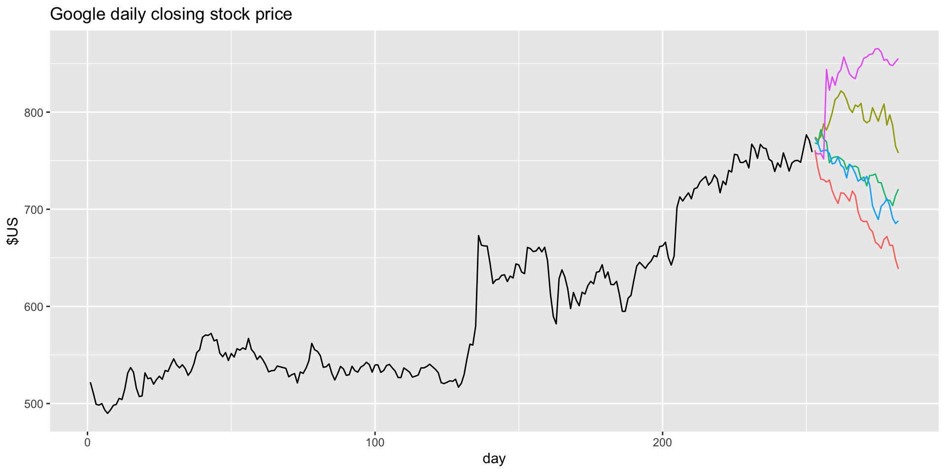
- Here are our five simulated futures plotted:
Bootstrap prediction intervals demonstration
- Here are our five simulated futures plotted:
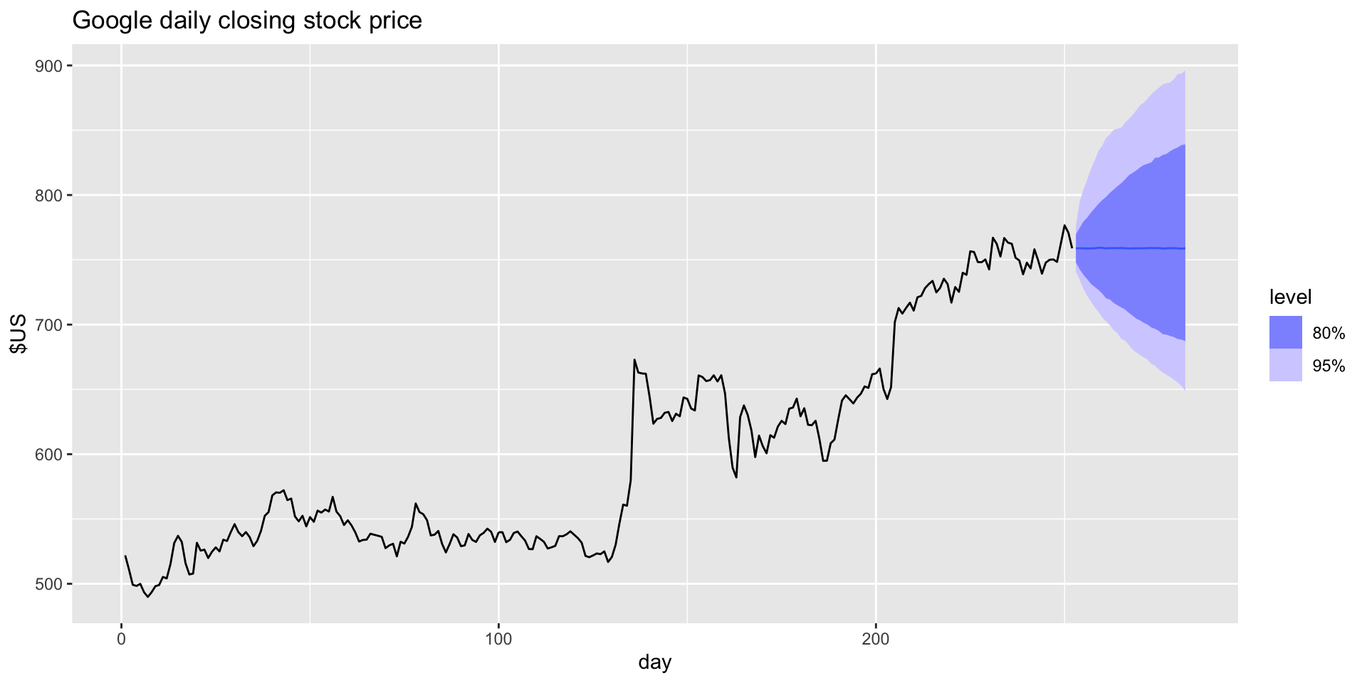
Bootstrap prediction intervals: bootstrapped distribution
- With these we can manufacture a “probability distribution”.
- Luckily there is a
bootstrapoption built intoforecast():
# A fable: 30 x 5 [1]
# Key:     Symbol, .model [1]
   Symbol .model         day        Close .mean
   <chr>  <chr>        <dbl>       <dist> <dbl>
 1 GOOG   NAIVE(Close)   253 sample[5000]  759.
 2 GOOG   NAIVE(Close)   254 sample[5000]  759.
 3 GOOG   NAIVE(Close)   255 sample[5000]  759.
 4 GOOG   NAIVE(Close)   256 sample[5000]  759.
 5 GOOG   NAIVE(Close)   257 sample[5000]  759.
 6 GOOG   NAIVE(Close)   258 sample[5000]  759.
 7 GOOG   NAIVE(Close)   259 sample[5000]  759.
 8 GOOG   NAIVE(Close)   260 sample[5000]  759.
 9 GOOG   NAIVE(Close)   261 sample[5000]  759.
10 GOOG   NAIVE(Close)   262 sample[5000]  759.
# ℹ 20 more rows
Bootstrap prediction intervals: bootstrapped distribution
- Note that the
.meancolumn is the mean of the bootstraps.
Bootstrapping in R
- Number of samples is controlled with the
timesoption:
bootstraps <- google_2015 |>
  model(NAIVE(Close)) |>
  forecast(h = 10, bootstrap = TRUE, times = 1000) |>
  hilo()
kable(bootstraps)| Symbol | .model | day | Close | .mean | 80% | 95% |
|---|---|---|---|---|---|---|
| GOOG | NAIVE(Close) | 253 | sample[1000] | 759.1838 | [747.9560, 771.8960]80 | [743.7060, 781.6654]95 |
| GOOG | NAIVE(Close) | 254 | sample[1000] | 759.2800 | [742.6378, 775.2679]80 | [733.9835, 796.0598]95 |
| GOOG | NAIVE(Close) | 255 | sample[1000] | 759.3544 | [739.1602, 780.3466]80 | [730.2132, 804.6933]95 |
| GOOG | NAIVE(Close) | 256 | sample[1000] | 759.5816 | [735.9287, 783.4072]80 | [725.6406, 818.4894]95 |
| GOOG | NAIVE(Close) | 257 | sample[1000] | 759.9708 | [733.4634, 786.7182]80 | [721.3592, 829.4516]95 |
| GOOG | NAIVE(Close) | 258 | sample[1000] | 759.1356 | [729.9575, 789.9693]80 | [715.2863, 833.4845]95 |
| GOOG | NAIVE(Close) | 259 | sample[1000] | 758.8663 | [728.2751, 793.5958]80 | [711.3703, 835.3340]95 |
| GOOG | NAIVE(Close) | 260 | sample[1000] | 759.1014 | [725.5190, 797.5592]80 | [707.3571, 837.5594]95 |
| GOOG | NAIVE(Close) | 261 | sample[1000] | 759.0371 | [722.4588, 799.1424]80 | [704.7527, 841.6002]95 |
| GOOG | NAIVE(Close) | 262 | sample[1000] | 758.8098 | [720.8937, 798.4185]80 | [703.2162, 843.4535]95 |
Exercise
- Create a 90% and 99% prediction interval for the forecast you produced last time.
- Create a bootstrapped forecast for the forecast you produced last time (try a bunch of different number of bootstraps)