Forecasting tools
BUS 323 Forecasting and Risk Analysis
Forecasting workflow
- Tidy
- Model-building
- Visualize
- Specify model
- Estimate model
- Evaluate model
- Repeat as necessary
- Forecast
Visualize
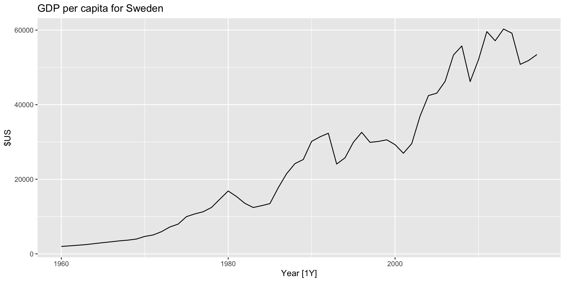
- Let’s plot Swedish GDP per capita from the
global_economydataset.
Visualize
- Let’s plot Swedish GDP per capita from the
global_economydataset.
Specify a model
- Linear trend:
Estimate the model
- To estimate the model, just specify the data you want to use:
Estimate the model
Evaluate the model
- Important to check how well your model has performed. More in a bit.
Forecast
- Use
forecast()! - To specify a timeframe for your forecast, use the
hoption:
# A fable: 789 x 5 [1Y]
# Key:     Country, .model [263]
   Country        .model       Year
   <fct>          <chr>       <dbl>
 1 Afghanistan    trend_model  2018
 2 Afghanistan    trend_model  2019
 3 Afghanistan    trend_model  2020
 4 Albania        trend_model  2018
 5 Albania        trend_model  2019
 6 Albania        trend_model  2020
 7 Algeria        trend_model  2018
 8 Algeria        trend_model  2019
 9 Algeria        trend_model  2020
10 American Samoa trend_model  2018
# ℹ 779 more rows
# ℹ 2 more variables: GDP_per_capita <dist>, .mean <dbl>
Forecast
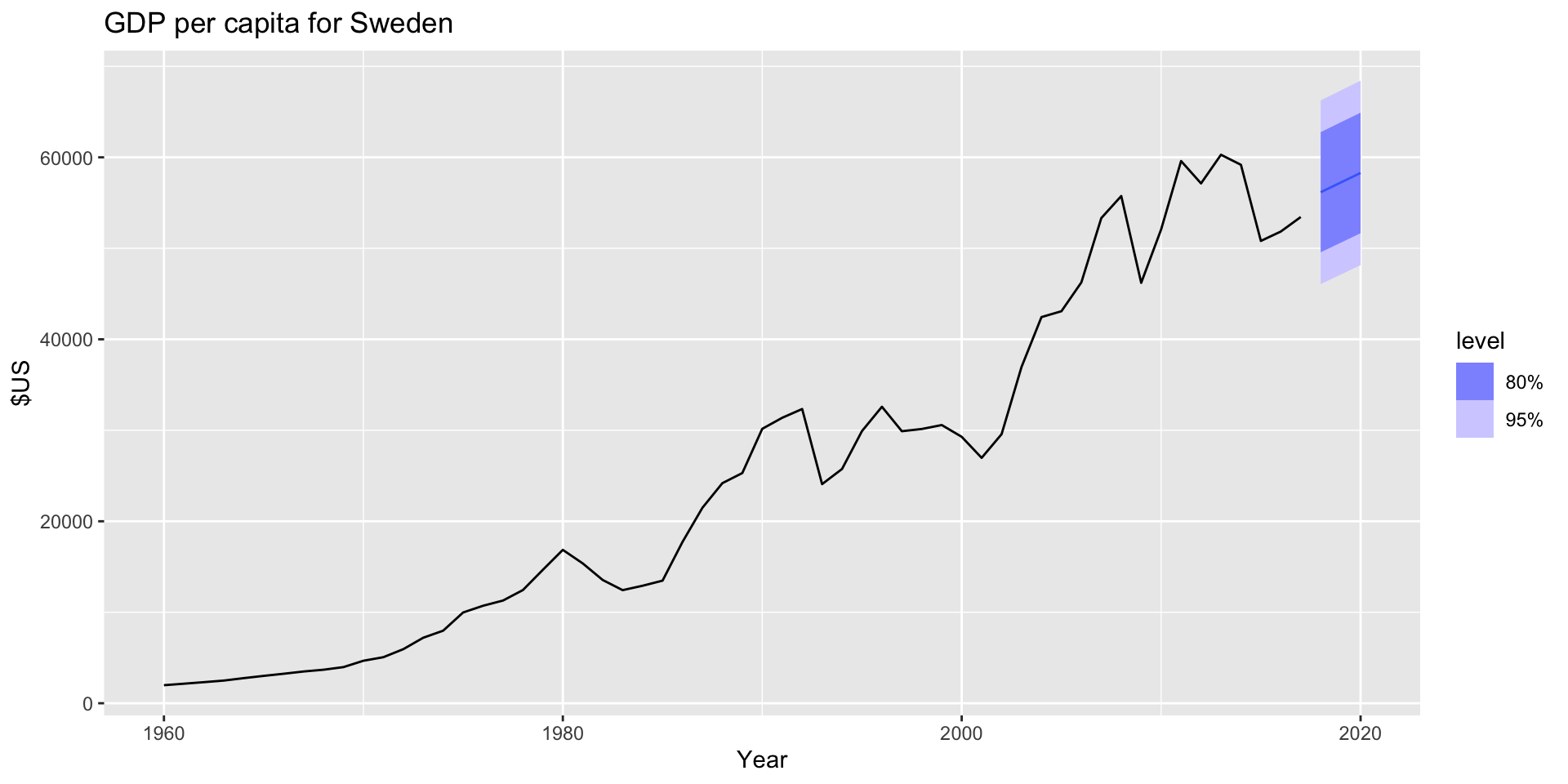
- The result is a “fable”, a forecast table. Each row corresponds to one forecast period. The
.meancolumn gives the average of the forecast distribution. - Plotting Sweden’s forecast:
Forecast
- The result is a “fable”, a forecast table. Each row corresponds to one forecast period. The
.meancolumn gives the average of the forecast distribution. - Plotting Sweden’s forecast:
More forecasting methods
- So far we have only talked about using regression to produce forecasts.
- Next we’ll dicsuss a few more simple forecasting methods.
Example dataset
- Use Australian clay brick production between 1970 and 2004 as example:
# A tsibble: 218 x 7 [1Q]
   Quarter  Beer Tobacco Bricks Cement Electricity   Gas
     <qtr> <dbl>   <dbl>  <dbl>  <dbl>       <dbl> <dbl>
 1 1956 Q1   284    5225    189    465        3923     5
 2 1956 Q2   213    5178    204    532        4436     6
 3 1956 Q3   227    5297    208    561        4806     7
 4 1956 Q4   308    5681    197    570        4418     6
 5 1957 Q1   262    5577    187    529        4339     5
 6 1957 Q2   228    5651    214    604        4811     7
 7 1957 Q3   236    5317    227    603        5259     7
 8 1957 Q4   320    6152    222    582        4735     6
 9 1958 Q1   272    5758    199    554        4608     5
10 1958 Q2   233    5641    229    620        5196     7
# ℹ 208 more rows
Example dataset
- Use
filter_index()to specify a range of the index to filter by:
# A tsibble: 140 x 7 [1Q]
   Quarter  Beer Tobacco Bricks Cement Electricity   Gas
     <qtr> <dbl>   <dbl>  <dbl>  <dbl>       <dbl> <dbl>
 1 1970 Q1   387    6807    386   1049       12328    12
 2 1970 Q2   357    7612    428   1134       14493    18
 3 1970 Q3   374    7862    434   1229       15664    23
 4 1970 Q4   466    7126    417   1188       13781    20
 5 1971 Q1   410    7255    385   1058       13299    19
 6 1971 Q2   370    8076    433   1209       15230    23
 7 1971 Q3   379    8405    453   1199       16667    28
 8 1971 Q4   487    7974    436   1253       14484    24
 9 1972 Q1   419    6500    399   1070       13838    24
10 1972 Q2   378    7119    461   1282       15919    34
# ℹ 130 more rows
Example dataset
- Use
select()to restrict attention only toBricks:
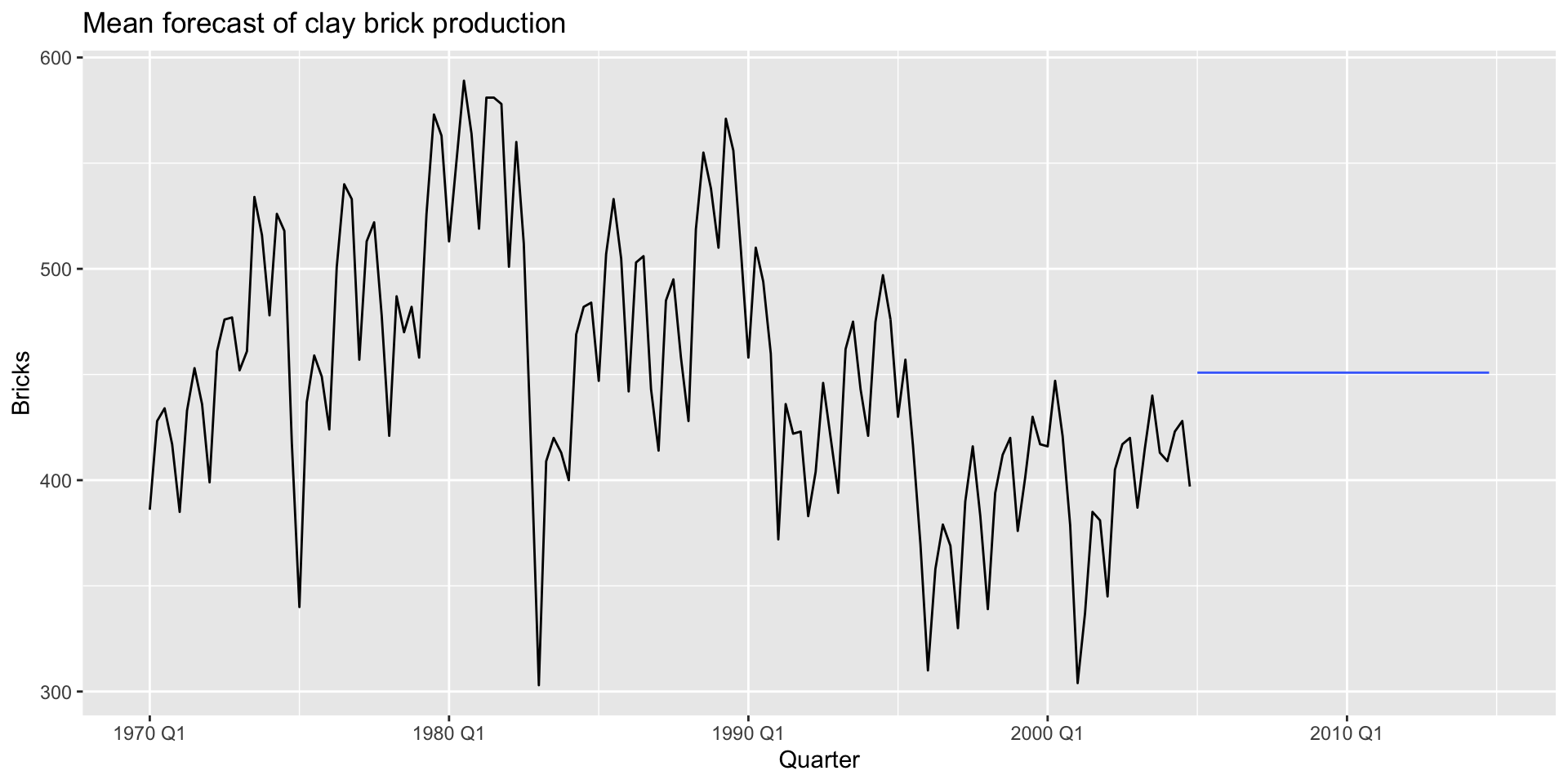
Mean method
- Use the mean of the historical data to forecast forward.
- The forecast estimate for a time series \(y\) \(h\) periods beyond the final observed period \(T\): \[ \hat{y}_{T+h|T} = \bar{y} = \frac{(y_{1} + ... + y_{t})}{T} \]
Mean method
- The function
model(MEAN())allows us to implement the mean method easily:
Mean method: forecasting
- The function
model(MEAN())allows us to implement the mean method easily:
Mean method: plotting
Mean method: plotting
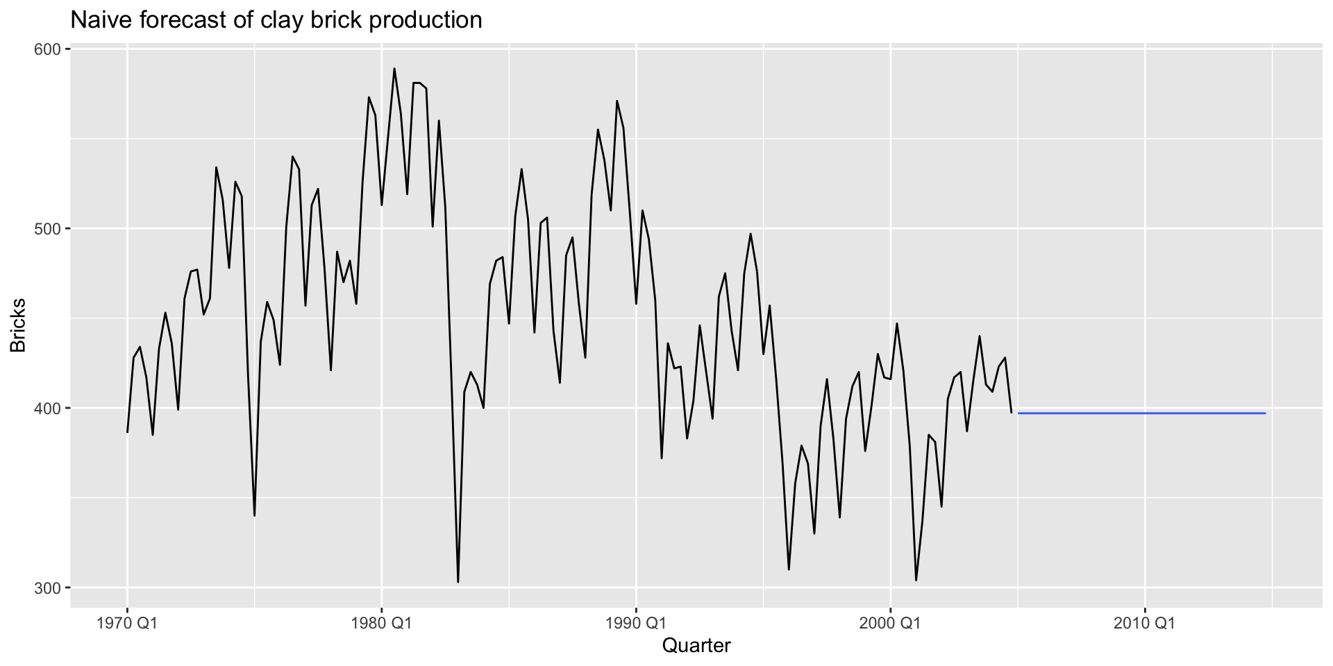
Naïve method
- Use value of last observation: \[ \hat{y}_{T+h | T} = y_{T} \]
Naïve method
- Use value of last observation: \[ \hat{y}_{T+h | T} = y_{T} \]
- AKA random walk forecasts.
Naïve implementation
- Implement with
model(NAIVE()):
Naïve forecast
- Implement with
model(NAIVE()):
Naïve plotting
- Implement with
model(NAIVE()):
Naïve plotting
- Implement with
model(NAIVE()):
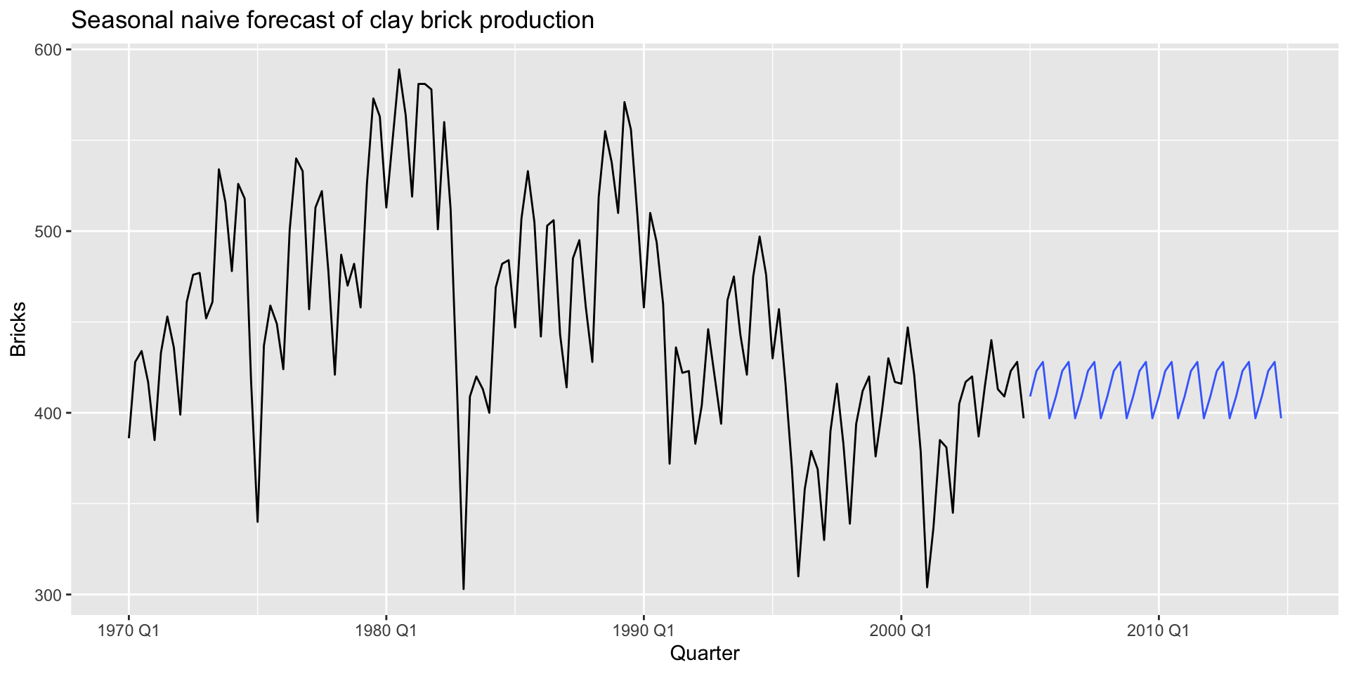
Seasonal naïve method
- Use value of last within-season observation: \[
\hat{y}_{T+h | T} = y_{T+h-m(k+1)}
\]
- \(m\): seasonal period
- \(k\): number of years in forecast prior to \(T+h\)
Seasonal naïve implementation
- Implement with
model(SNAIVE()):
Seasonal naïve forecast
# A fable: 40 x 4 [1Q]
# Key:     .model [1]
   .model                           Quarter
   <chr>                              <qtr>
 1 "SNAIVE(Bricks ~ lag(\"year\"))" 2005 Q1
 2 "SNAIVE(Bricks ~ lag(\"year\"))" 2005 Q2
 3 "SNAIVE(Bricks ~ lag(\"year\"))" 2005 Q3
 4 "SNAIVE(Bricks ~ lag(\"year\"))" 2005 Q4
 5 "SNAIVE(Bricks ~ lag(\"year\"))" 2006 Q1
 6 "SNAIVE(Bricks ~ lag(\"year\"))" 2006 Q2
 7 "SNAIVE(Bricks ~ lag(\"year\"))" 2006 Q3
 8 "SNAIVE(Bricks ~ lag(\"year\"))" 2006 Q4
 9 "SNAIVE(Bricks ~ lag(\"year\"))" 2007 Q1
10 "SNAIVE(Bricks ~ lag(\"year\"))" 2007 Q2
# ℹ 30 more rows
# ℹ 2 more variables: Bricks <dist>, .mean <dbl>
Seasonal naïve plotting
Drift method
- Naïve method allowing for “drift”
Drift method
- Naïve method allowing for “drift”
- Increase/decrease in forecast over time
Drift method
- Naïve method allowing for “drift”
- Increase/decrease in forecast over time
- Drift set to average observed change
Drift method
- Naïve method allowing for “drift”
- Increase/decrease in forecast over time
- Drift set to average observed change
- Forecast for \(T+h\): \[ \hat{y}_{T+h | T} = y_{T} + h\frac{\sum_{t=2}^{T} (y_{t} - y_{t-1})}{T-2} = y_{T} + h(\frac{y_{T}-y_{1}}{T-1}) \]
Drift implementation
- Use
model(RW()):
Drift forecast
# A fable: 40 x 4 [1Q]
# Key:     .model [1]
   .model               Quarter
   <chr>                  <qtr>
 1 RW(Bricks ~ drift()) 2005 Q1
 2 RW(Bricks ~ drift()) 2005 Q2
 3 RW(Bricks ~ drift()) 2005 Q3
 4 RW(Bricks ~ drift()) 2005 Q4
 5 RW(Bricks ~ drift()) 2006 Q1
 6 RW(Bricks ~ drift()) 2006 Q2
 7 RW(Bricks ~ drift()) 2006 Q3
 8 RW(Bricks ~ drift()) 2006 Q4
 9 RW(Bricks ~ drift()) 2007 Q1
10 RW(Bricks ~ drift()) 2007 Q2
# ℹ 30 more rows
# ℹ 2 more variables: Bricks <dist>, .mean <dbl>
Drift plotting
Drift plotting
