Time series decomposition

BUS 323 Forecasting and Risk Analysis

Time series components - additive decomposition

If we assume an additive decomposition, we can write: \[ y_{t} = S_{t} + T_{t} + R_{t} \] where \(y_{t}\) represents a time series variable’s value at period \(t\); \(S\) represents the seasonal component of the series; \(T\) represents the trend-cycle component of the series; and \(R\) represents the remainder component of the series.

Time series components - additive decomposition

If we assume an additive decomposition, we can write: \[ y_{t} = S_{t} + T_{t} + R_{t} \] where \(y_{t}\) represents a time series variable’s value at period \(t\); \(S\) represents the seasonal component of the series; \(T\) represents the trend-cycle component of the series; and \(R\) represents the remainder component of the series.
Additive decomposition is appropriate if the magnitude of the seasonal fluctuations or the variation around the trend-cycle does not vary with \(t\).

Time series components - multiplicative decomposition

A multiplicative decomposition would be written: \[ y_{t} = S_{t} \times T_{t} \times R_{t} \] where all objects are as defined above.

Time series components - multiplicative decomposition

A multiplicative decomposition would be written: \[ y_{t} = S_{t} \times T_{t} \times R_{t} \] where all objects are as defined above.
Multiplicative decompositionis appropriate when the variation in the seasonal patter or the variation around the trend-cycle appears proportional to \(t\).

Time series components - multiplicative decomposition

Note that \(t_{t} = S_{t} \times T_{t} \times R_{t}\) is equivalent to \[ log(y_{t}) = log(S_{t}) + log(T_{t}) + log(R_{t}) \]
So in the case of a multiplicative decomposition, it is standard to transform the series such that the variation appears stable over time, then apply an additive decomposition.

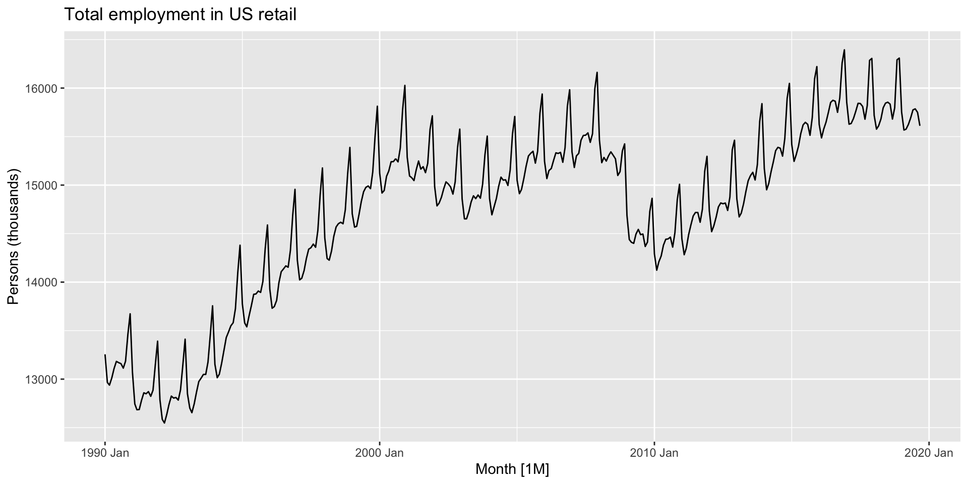
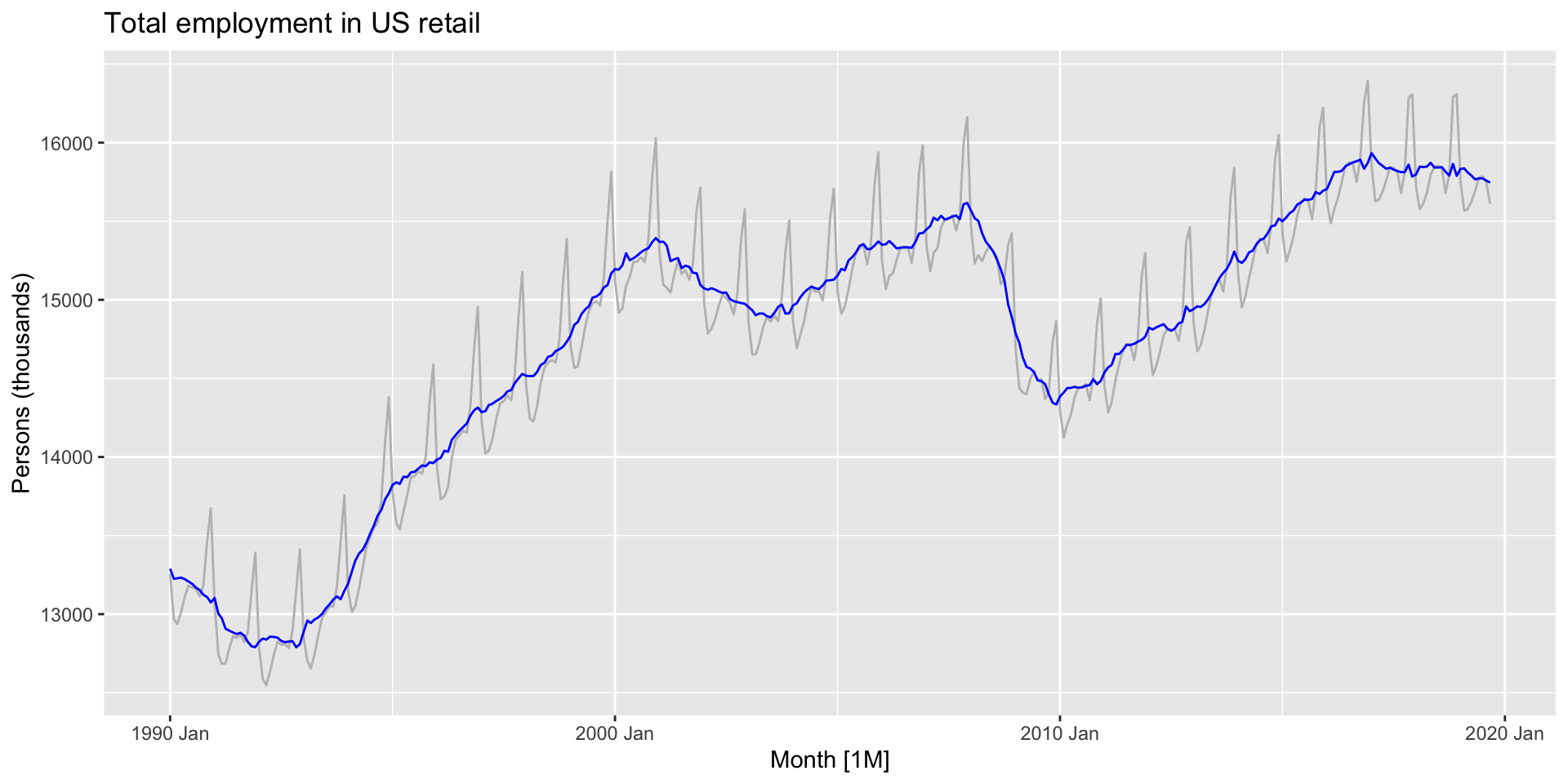
Example: US retail employment

We’ll talk about decomposition methods soon, but let’s see the benefit first.
Here’s a time plot of US retail employment we’ll decompose.

library(fpp3)
us_retail_employment <- us_employment |>
  filter(year(Month) >= 1990, Title == "Retail Trade") |>
  select(-Series_ID)
autoplot(us_retail_employment, Employed) +
  labs(y = "Persons (thousands)",
       title = "Total employment in US retail")

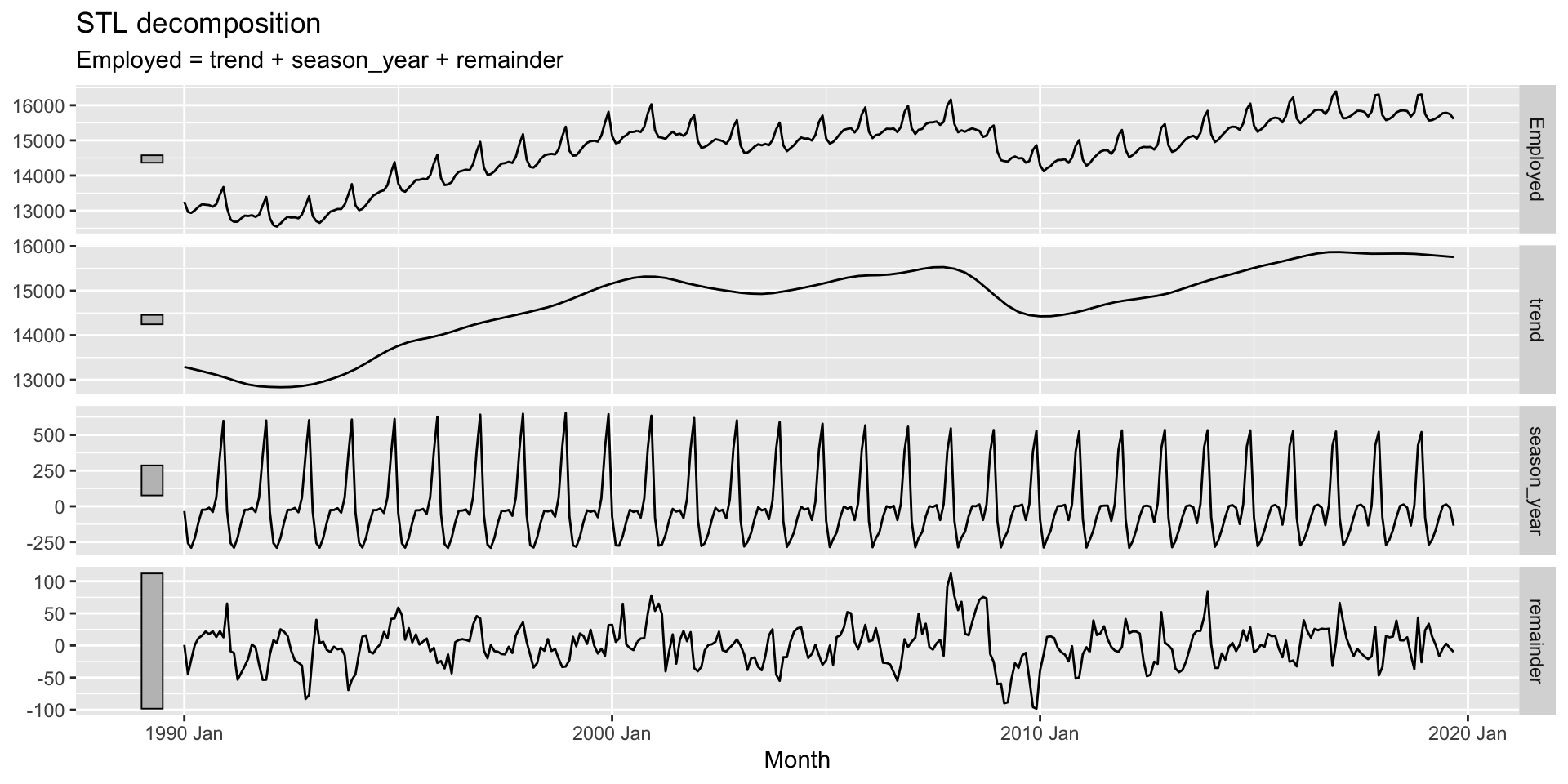
Example: US retail employment

Here’s the plot with just the trend-cycle component:

Example: US retail employment

Here’s a plot with all three decomposed components:

Example: US retail employment

“Seasonally adjusted” data have the seasonal component of the series removed.

Example: US retail employment

“Seasonally adjusted” data have the seasonal component of the series removed.
- For additive decomposition: \(y_{t} - S_{t}\)

Example: US retail employment

“Seasonally adjusted” data have the seasonal component of the series removed.
- For additive decomposition: \(y_{t} - S_{t}\)
- For multiplicative decomposition: \(\frac{y_{t}}{S_{t}}\)

Example: US retail employment

“Seasonally adjusted” data have the seasonal component of the series removed.
- For additive decomposition: \(y_{t} - S_{t}\)
- For multiplicative decomposition: \(\frac{y_{t}}{S_{t}}\)
Here’s a seasonally adjusted retail employment time plot:

Example: US retail employment

Moving average models

MA models are used for decomposing the trend-cycle component of a series.

Moving average models

MA models are used for decomposing the trend-cycle component of a series.
A moving average of order \(m\) can be written: \[ \hat{T}_{t} = \frac{1}{m} \sum_{j = -k}^{k} y_{t+j} \] where \(m=2k+1\).

Moving average models

MA models are used for decomposing the trend-cycle component of a series.
A moving average of order \(m\) can be written: \[ \hat{T}_{t} = \frac{1}{m} \sum_{j = -k}^{k} y_{t+j} \] where \(m=2k+1\).
Suppose \(k=1\). Expand the above expression out to gain some intuition about it.

Moving average models

MA models are used for decomposing the trend-cycle component of a series.
A moving average of order \(m\) can be written: \[ \hat{T_{t}} = \frac{1}{m} \sum_{j = -k}^{k} y_{t+j} \] where \(m=2k+1\).
Suppose \(k=1\). Expand this expression out to gain some intuition about it.

Moving averages

\[ \hat{T_{t}} = \frac{y_{t-1} + y_{t} + y_{t+1}}{2} \] The above is a MA(2) model, or a 2-MA model.

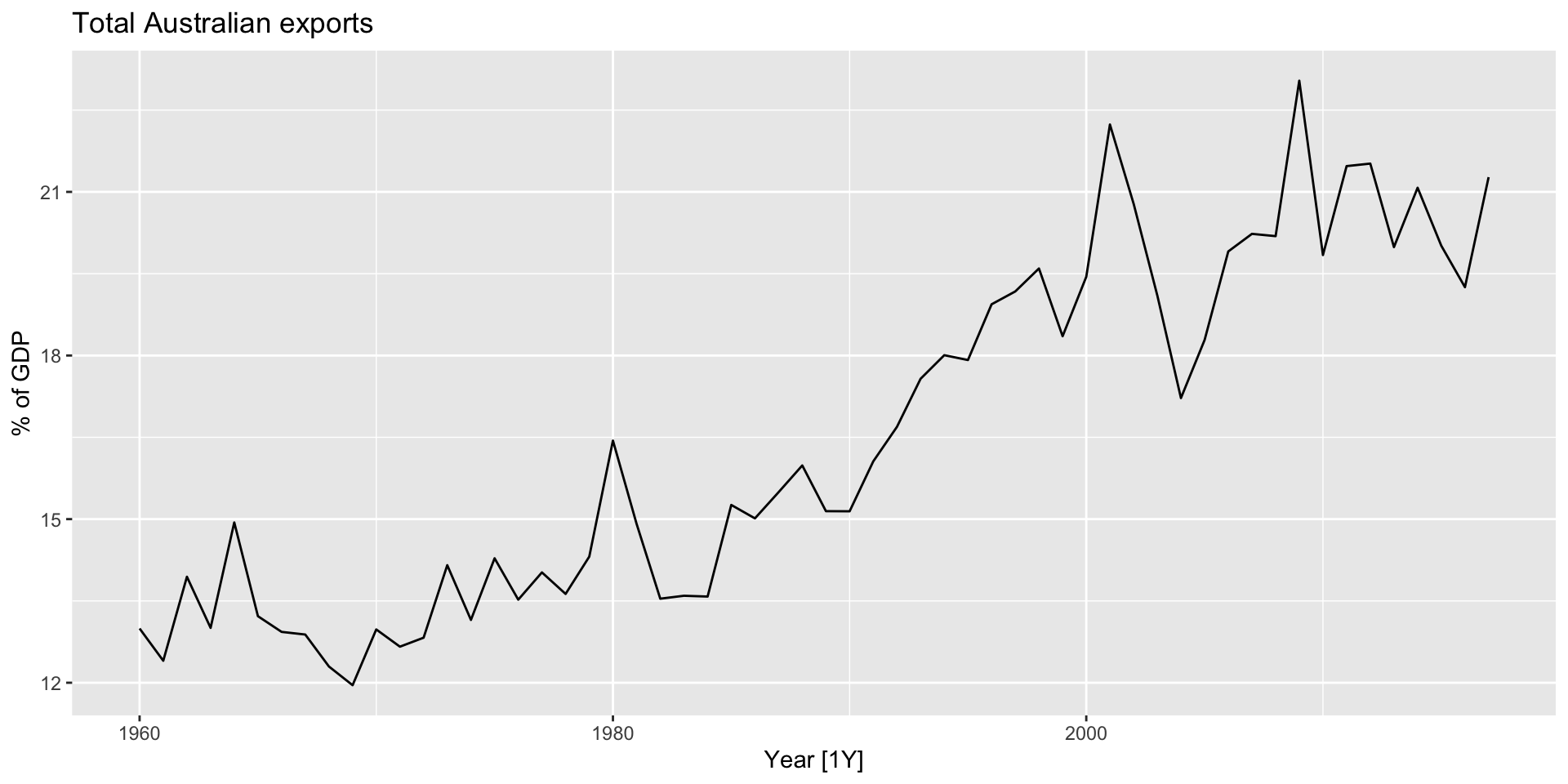
Moving averages: application

Make an autoplot of Australian exports from the global_economy dataset:

aus_economy <- global_economy |>
  filter(Country == "Australia")
aus_economy |>
  autoplot(Exports) +
  labs(y = "% of GDP", title = "Total Australian exports")

Moving averages: application

We can execute a 5-MA transformation manually with an iterative loop. First, we’ll define the parameters:

k <- 2  
m <- 2 * k + 1

Moving averages: application

Next, make a vector we’ll put the 5-MA transformation in:

aus_economy$ma_5 <- rep(NA, length(aus_economy$Exports))

Moving averages: application

Finally, we can make a loop to feed the 5-period average of Exports into each observation in ma_5:

for (i in (k + 1):(length(aus_economy$Exports) - k)) {
  aus_economy$ma_5[i] <- mean(aus_economy$Exports[(i - k):(i + k)])
}

aus_economy |>
  select(Exports, ma_5) |>
    head()

# A tsibble: 6 x 3 [1Y]
  Exports  ma_5  Year
    <dbl> <dbl> <dbl>
1    13.0  NA    1960
2    12.4  NA    1961
3    13.9  13.5  1962
4    13.0  13.5  1963
5    14.9  13.6  1964
6    13.2  13.4  1965

Moving averages: application

We can also do this automatically using slide_dbl() from the slider package.
- The function applies a given function (for us, it will be mean) to “sliding” time windows.

Moving averages: application

We can also do this automatically using slide_dbl() from the slider package.

The function applies a given function (for us, it will be mean) to “sliding” time windows.

aus_economy |>
  mutate(
    ma5 = slider::slide_dbl(Exports, mean,
                             .before = 2, 
                             .after = 2,
                             .complete = TRUE)
  ) |>
    select(Exports, ma5) |>
      head()

# A tsibble: 6 x 3 [1Y]
  Exports   ma5  Year
    <dbl> <dbl> <dbl>
1    13.0  NA    1960
2    12.4  NA    1961
3    13.9  13.5  1962
4    13.0  13.5  1963
5    14.9  13.6  1964
6    13.2  13.4  1965

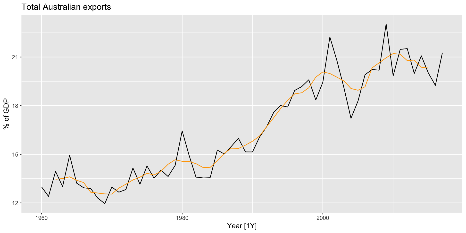
Moving averages: application

Let’s plot the trend-cycle component estimates from our 5-MA object along with the time plot of exports:

aus_economy |>
  autoplot(Exports) +
  geom_line(aes(y = ma_5), colour = "orange") +
  labs(y = "% of GDP",
       title = "Total Australian exports")

Moving averages of moving averages

If you use an even-order MA, you can take another even-order MA of the MA to make the whole process symmetric.

Moving averages of moving averages

If you use an even-order MA, you can take another even-order MA of the MA to make the whole process symmetric.
Consider a 4-MA followed by a 2-MA: \[ \hat{T_{t}} = \frac{1}{2} [\frac{1}{4} (y_{t-1} + y_{t} + y_{t+1} + y_{t+2}) + \frac{1}{4} (y_{t-2} + y_{t-1} + y_{t} + y_{t+1})] \\ = \frac{1}{8} y_{t-2} + \frac{1}{4} y_{t-1} + \frac{1}{4} y_{t} + \frac{1}{4} y_{t+1} + \frac{1}{8} y_{t+2} \] ## Moving averages of moving averages
If you use an even-order MA, you can take another even-order MA of the MA to make the whole process symmetric.
Consider a 4-MA followed by a 2-MA: \[ \hat{T_{t}} = \frac{1}{2} [\frac{1}{4} (y_{t-1} + y_{t} + y_{t+1} + y_{t+2}) + \frac{1}{4} (y_{t-2} + y_{t-1} + y_{t} + y_{t+1})] \\ = \frac{1}{8} y_{t-2} + \frac{1}{4} y_{t-1} + \frac{1}{4} y_{t} + \frac{1}{4} y_{t+1} + \frac{1}{8} y_{t+2} \]
Why might this be useful?

Estimating the trend-cycle with seasonal data

When applying the 2x4-MA to quarterly data, each quarter is given equal weight. As a result the seasonal variation will be averaged out.

Estimating the trend-cycle with seasonal data

When applying the 2x4-MA to quarterly data, each quarter is given equal weight. As a result the seasonal variation will be averaged out.
- You can use a 2x12-MA to estimate the trend-cycle of monthly data with annual seasonality.

Estimating the trend-cycle with seasonal data

When applying the 2x4-MA to quarterly data, each quarter is given equal weight. As a result the seasonal variation will be averaged out.
- You can use a 2x12-MA to estimate the trend-cycle of monthly data with annual seasonality.
- A 7-MA to estimate the trend-cycle of daily data with weekly seasonality.

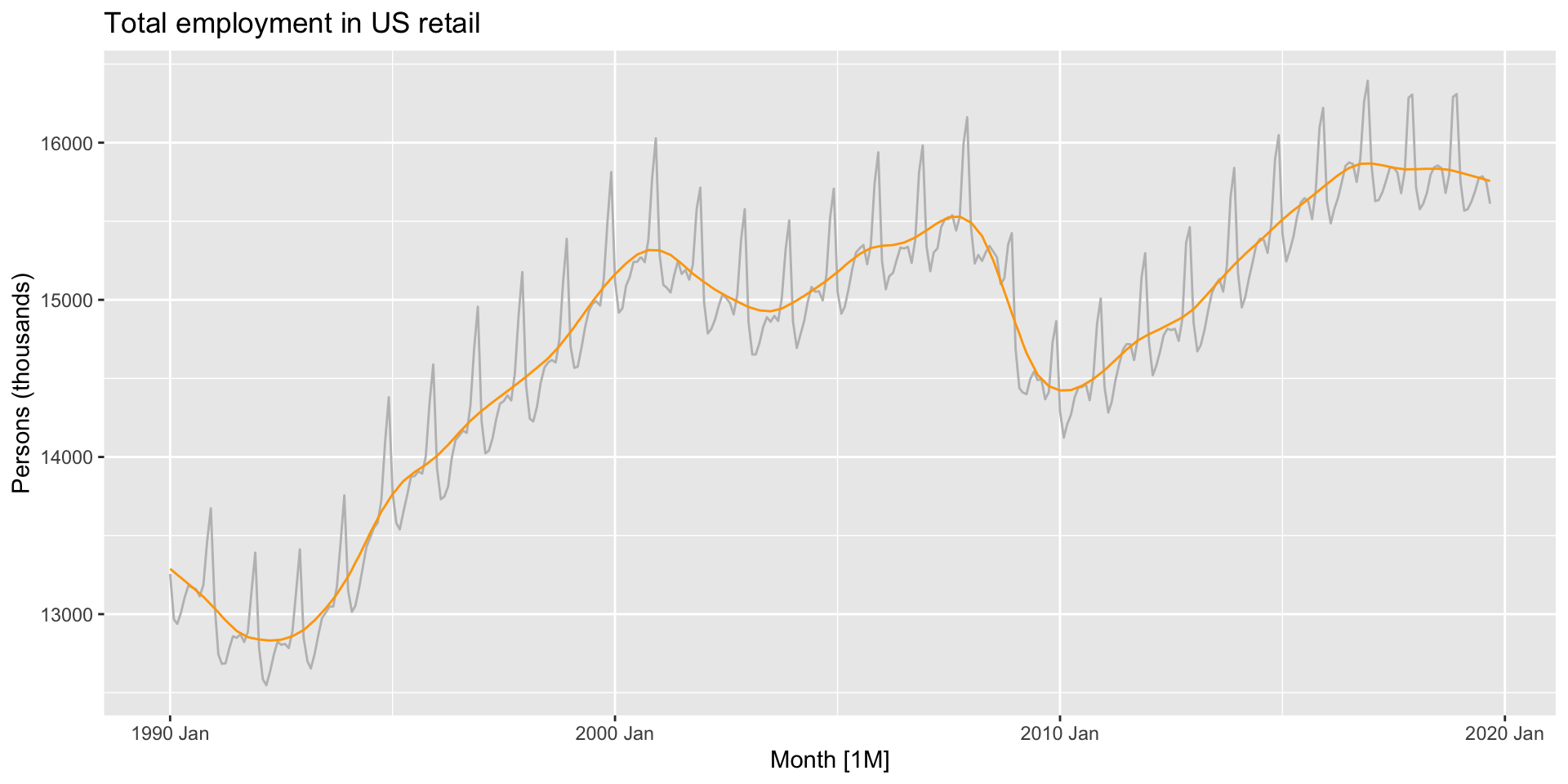
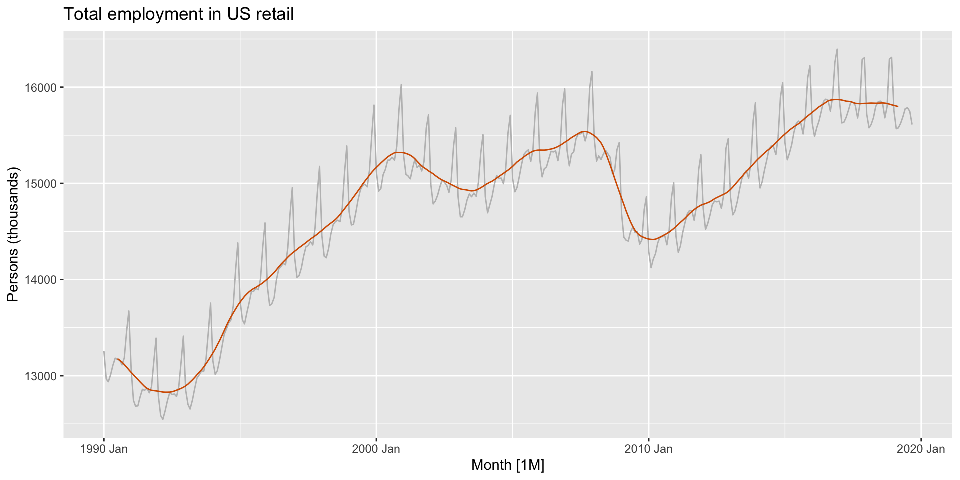
Example: US retail employment

us_retail_employment_ma <- us_retail_employment |>
  mutate(
    `12-MA` = slider::slide_dbl(Employed, mean,
                .before = 5, .after = 6, .complete = TRUE),
    `2x12-MA` = slider::slide_dbl(`12-MA`, mean,
                .before = 1, .after = 0, .complete = TRUE)
  )
us_retail_employment_ma |>
  autoplot(Employed, colour = "gray") +
  geom_line(aes(y = `2x12-MA`), colour = "#D55E00") +
  labs(y = "Persons (thousands)",
       title = "Total employment in US retail")

Example: US retail employment

Classical decomposition

Assume seasonal period \(m\).
Assume constant seasonal component across time.

Classical decomposition

Assume seasonal period \(m\).
Assume constant seasonal component across time.

If \(m\) is even, compute \(\hat{T_{t}}\) using a \(2 \times m\)-MA. If \(m\) is odd, compute \(\hat{T_{t}}\) using a \(m\)-MA.

Classical decomposition

Assume seasonal period \(m\).
Assume constant seasonal component across time.

If \(m\) is even, compute \(\hat{T_{t}}\) using a \(2 \times m\)-MA. If \(m\) is odd, compute \(\hat{T_{t}}\) using a \(m\)-MA.
Calculate the detrended series \(y_{t} - \hat{T_{t}}\).

Classical decomposition

Assume seasonal period \(m\).
Assume constant seasonal component across time.

If \(m\) is even, compute \(\hat{T_{t}}\) using a \(2 \times m\)-MA. If \(m\) is odd, compute \(\hat{T_{t}}\) using a \(m\)-MA.
Calculate the detrended series \(y_{t} - \hat{T_{t}}\).
Average the within-season detrended values to obtain \(\hat{S_{t}}\).

Classical decomposition

Assume seasonal period \(m\).
Assume constant seasonal component across time.

If \(m\) is even, compute \(\hat{T_{t}}\) using a \(2 \times m\)-MA. If \(m\) is odd, compute \(\hat{T_{t}}\) using a \(m\)-MA.
Calculate the detrended series \(y_{t} - \hat{T_{t}}\).
Average the within-season detrended values to obtain \(\hat{S_{t}}\).
Calculate the remainder component \(\hat{R_{t}} = y_{t} - \hat{T_{t}} - \hat{S_{t}}\).

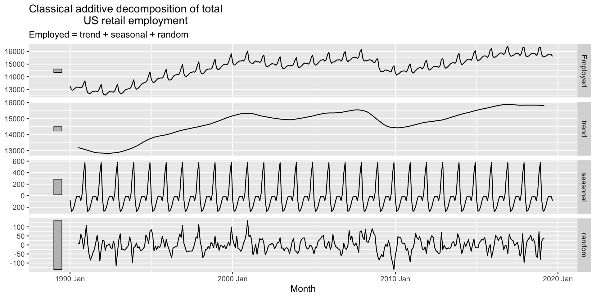
Classical decomposition example

Luckily there is an R function that does all this for us: classical_decomposition():

us_retail_employment |>
  model(
    classical_decomposition(Employed, type = "additive")
  ) |>
  components() |>
  autoplot() +
  labs(title = "Classical additive decomposition of total
                  US retail employment")

Classical decomposition example

Luckily there is an R function that does all this for us: classical_decomposition():

Classical decomposition limitations

Can’t estimate the trend-cycle for the first few and last few observations.

Classical decomposition limitations

Can’t estimate the trend-cycle for the first few and last few observations.
The trend-cycle estimate tends to over-smooth rapid rises and falls.

Classical decomposition limitations

Can’t estimate the trend-cycle for the first few and last few observations.
The trend-cycle estimate tends to over-smooth rapid rises and falls.
The assumption that the seasonal component remans constant over time is often unrealistic.

Classical decomposition limitations

Can’t estimate the trend-cycle for the first few and last few observations.
The trend-cycle estimate tends to over-smooth rapid rises and falls.
The assumption that the seasonal component remans constant over time is often unrealistic.
Not robust to outliers.

STL decomposition

STL: “Seasonal and Trend decomposition using Loess”

STL decomposition

STL: “Seasonal and Trend decomposition using Loess”
- loess: a non-parametric local linear regression method for estimating nonlinear relationships

STL decomposition

STL: “Seasonal and Trend decomposition using Loess”
- loess: a non-parametric local linear regression method for estimating nonlinear relationships
- Note that STL only works for aditive decompositions

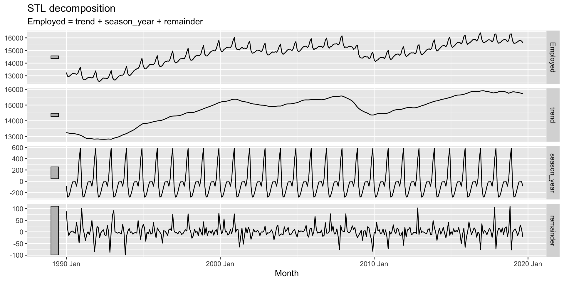
STL decomposition: example

Try out the following:

us_retail_employment |>
  model(
    STL(Employed)
  ) |>
    components() |>
      autoplot()

STL decomposition: example

STL decomposition: parameters

Trend-cycle window: trend(window = x)

STL decomposition: parameters

Trend-cycle window: trend(window = x)
- The number of consecutive observations to use when estimating the trend-cycle component

STL decomposition: parameters

Trend-cycle window: trend(window = x)
- The number of consecutive observations to use when estimating the trend-cycle component
Seasonal window: season(window = x)

STL decomposition: parameters

Trend-cycle window: trend(window = x)
- The number of consecutive observations to use when estimating the trend-cycle component
Seasonal window: season(window = x)
- The number of consecutive years to use in estimating each value in the seasonal component.

STL decomposition: parameters

Trend-cycle window: trend(window = x)
- The number of consecutive observations to use when estimating the trend-cycle component
Seasonal window: season(window = x)
- The number of consecutive years to use in estimating each value in the seasonal component.
- season(window = 'periodic') forces the component to be identical across years.

STL decomposition: parameters

Trend-cycle window: trend(window = x)
- The number of consecutive observations to use when estimating the trend-cycle component
Seasonal window: season(window = x)
- The number of consecutive years to use in estimating each value in the seasonal component.
- season(window = 'periodic') forces the component to be identical across years.
Robustness: robust = TRUE
- Reduces the influence of outliers by using robust loess.

STL decomposition: example, again

Try the following:

us_retail_employment |>
  model(
    STL(Employed ~ trend(window = 7) +
                   season(window = "periodic"),
    robust = TRUE)) |>
  components() |>
  autoplot()