Transformations

BUS 323 Forecasting and Risk Analysis

Three components for decomposition

1. Trend-cycle component
2. Seasonal component
3. Remainder component

Why decompose?

• Improve understanding
• Improve forecast accuracy
• Often, need to transform the series first

Calendar adjustments

• Some variation due to calendar effects. We may want to remove that variation to make the patterns more predictable.
• e.g. Some months have 30 days, some have 31. Some have 28. Some have 29!
  • If we computed total sales per month, some months would have “bonus” days, making them look more productive.
  • One possible adjustment: average sales per day.

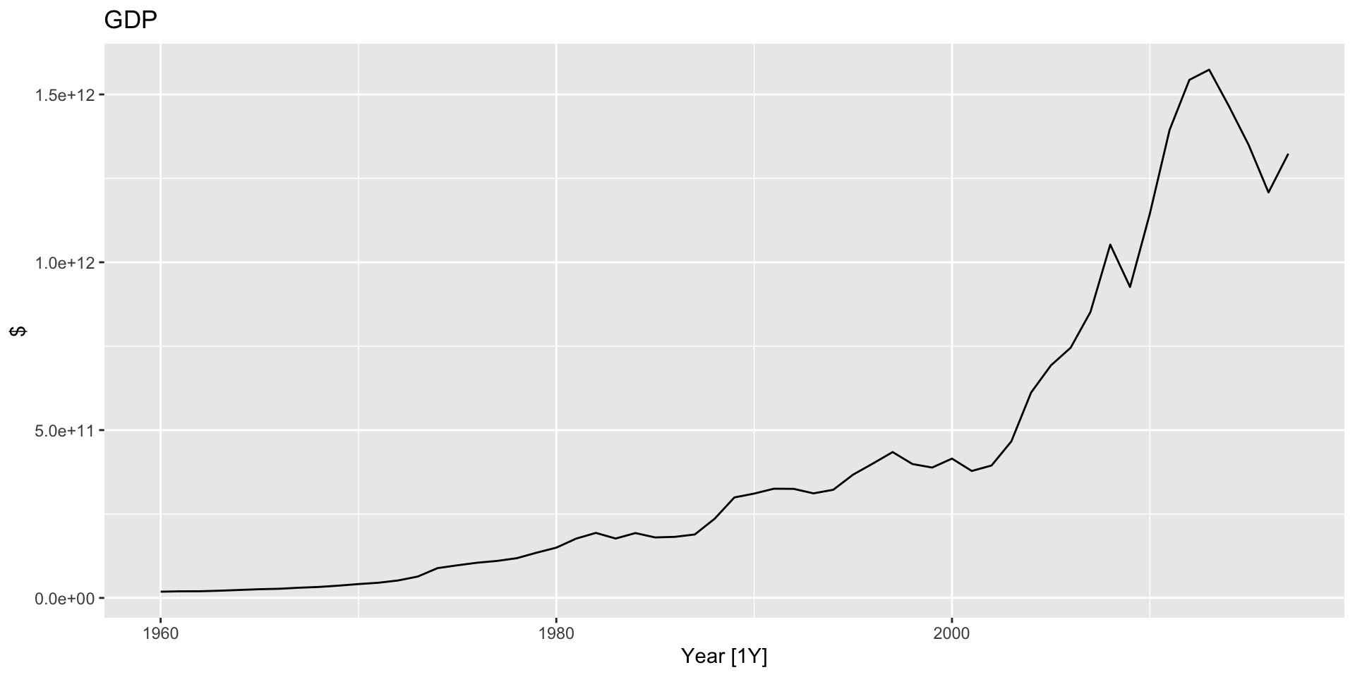
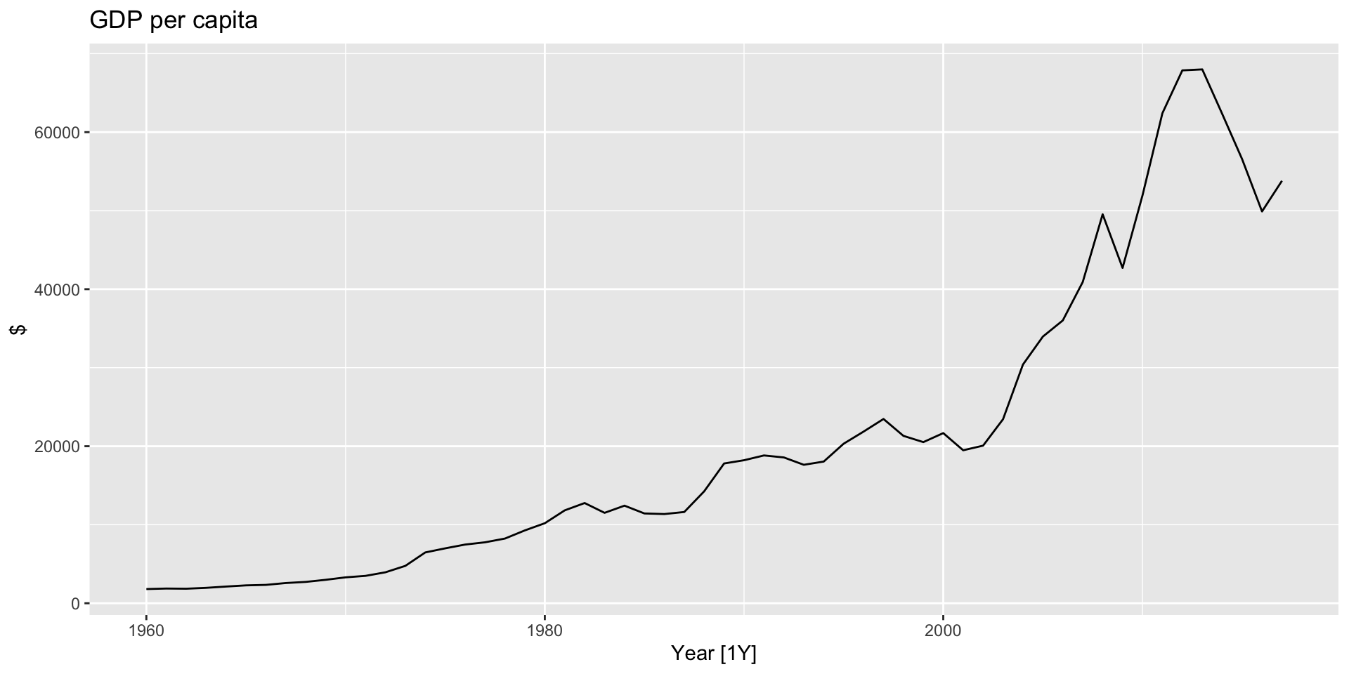
Population adjustments

• Some data series are affected by population changes.We can alter them to give per-capita data.
• e.g. GDP. What would GDP per capita reflect that GDP on its own does not?

Population adjustments

• Some data series are affected by population changes.We can alter them to give per-capita data.
• e.g. GDP. What would GDP per capita reflect that GDP on its own does not?
• Use global_economy to make a time plot of US GDP and US per-capita GDP.

Population adjustments

• Some data series are affected by population changes.We can alter them to give per-capita data.
• e.g. GDP. What would GDP per capita reflect that GDP on its own does not?
• Use global_economy to make a time plot of Australia GDP and per-capita GDP.

Population adjustments: GDP time plot

library(fpp3)
global_economy |>
  filter(Country == "Australia") |>
  autoplot(GDP) +
  labs(title = "GDP", y = "$")

Population adjustments: GDP time plot

Population adjustments: GDP per capita time plot

library(fpp3)
global_economy |>
  filter(Country == "Australia") |>
  autoplot(GDP/Population) +
  labs(title = "GDP per capita", y = "$")

Population adjustments: GDP per capita time plot

Inflation adjustments

• Data which are affected by the value of money should be adjusted before modeling.
  • e.g. a $0.99 Arizona Iced Tea today is not the same as a $0.99 Arizona Iced Tea in 2010.

Inflation adjustments

• To adjust, use a price index.
  • Let \(z_{t}\) represent the price index in year \(t\) and \(y_{t}\) represent the price of Arizona Iced Tea in year \(t\).
  • Then the price of Arizona Iced Tea in 2000 dollars would be: \(x_{t} = \frac{y_{t}}{z_{t}} \times z_{2000}\)
• The Consumer Price Index (CPI) is commonly used for this. The CPI is equal to 100 in the base year.

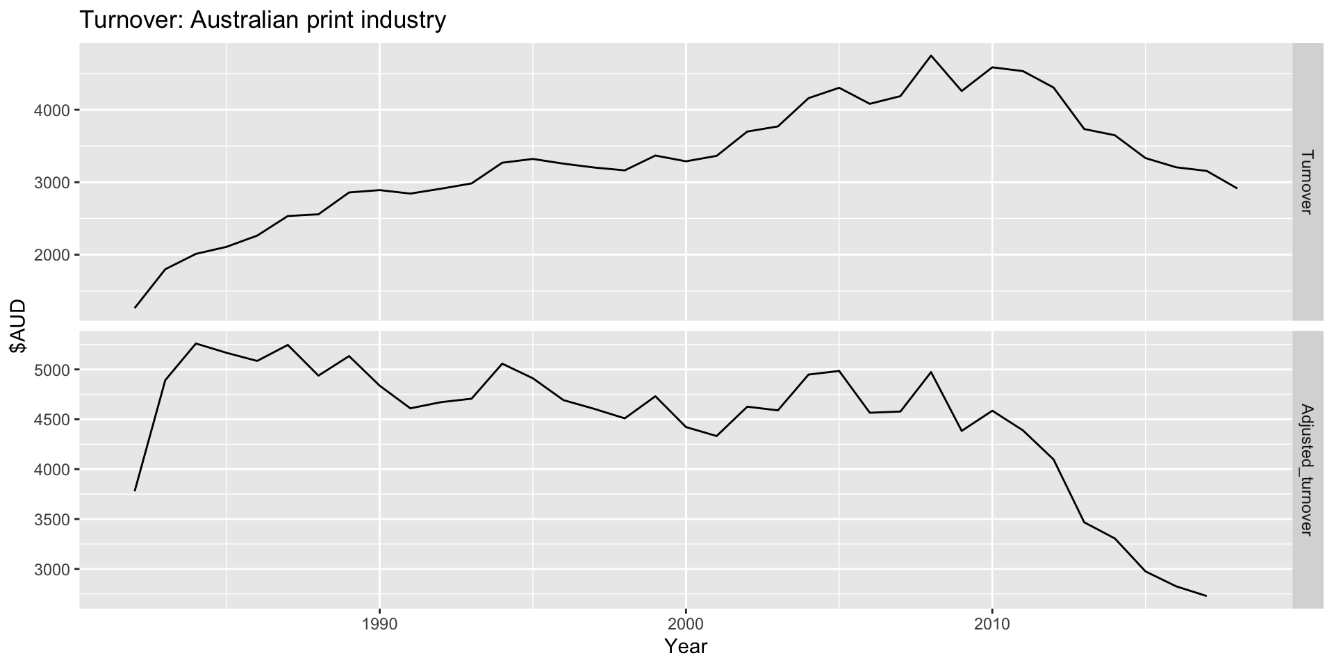
Inflation adjustments: Australia retail

• The aus_retail dataset gives retail turnover in $Million AUD. Let’s inflation-adjust that series.
• In particular, let’s inflation-adjust total retail turnover across states by year for a certain industry. I’ll look “Newspaper and book retailing”. Use whatever industry you like. The first step is to get total retail turnover by year for that industry:

print_retail <- aus_retail |>
  filter(Industry == "Newspaper and book retailing") |>
    group_by(Industry) |>
      index_by(Year = year(Month)) |>
        summarise(Turnover = sum(Turnover))

Inflation adjustments: Australia retail

• Next we’ll need to get our price index. We can grab the CPI from global_economy:

aus_economy <- global_economy |>
  filter(Code == "AUS")

Inflation adjustments: Australia retail

• Next we’ll need to use the CPI from aus_economy to inflation-adjust the values of Turnover from print_retail:

print_retail |>
  left_join(aus_economy, by = "Year") |>
    mutate(Adjusted_turnover = (Turnover/CPI)*100)

# A tsibble: 37 x 12 [1Y]
# Key:       Industry [1]
   Industry     Year Turnover Country Code      GDP Growth   CPI Imports Exports
   <chr>       <dbl>    <dbl> <fct>   <fct>   <dbl>  <dbl> <dbl>   <dbl>   <dbl>
 1 Newspaper …  1982    1263  Austra… AUS   1.94e11  3.33   33.4    16.8    13.5
 2 Newspaper …  1983    1800. Austra… AUS   1.77e11 -2.22   36.8    15.6    13.6
 3 Newspaper …  1984    2011. Austra… AUS   1.93e11  4.58   38.2    15.0    13.6
 4 Newspaper …  1985    2109. Austra… AUS   1.80e11  5.25   40.8    17.3    15.3
 5 Newspaper …  1986    2263. Austra… AUS   1.82e11  4.06   44.5    18.1    15.0
 6 Newspaper …  1987    2534. Austra… AUS   1.89e11  2.51   48.3    17.1    15.5
 7 Newspaper …  1988    2557. Austra… AUS   2.36e11  5.68   51.8    16.6    16.0
 8 Newspaper …  1989    2859. Austra… AUS   2.99e11  3.87   55.7    17.0    15.1
 9 Newspaper …  1990    2891. Austra… AUS   3.11e11  3.56   59.8    17.1    15.1
10 Newspaper …  1991    2843. Austra… AUS   3.25e11 -0.388  61.7    16.2    16.1
# ℹ 27 more rows
# ℹ 2 more variables: Population <dbl>, Adjusted_turnover <dbl>

Inflation adjustments: Australia retail

• For plotting, we’ll need to pivot turnover so that it’s indexed by whether it’s inflation-adjusted or not

print_retail |>
  left_join(aus_economy, by = "Year") |>
    mutate(Adjusted_turnover = (Turnover/CPI)*100) |>
      pivot_longer(c(Turnover, Adjusted_turnover), values_to = "Turnover")

# A tsibble: 74 x 12 [1Y]
# Key:       Industry, name [2]
   Industry   Year Country Code      GDP Growth   CPI Imports Exports Population
   <chr>     <dbl> <fct>   <fct>   <dbl>  <dbl> <dbl>   <dbl>   <dbl>      <dbl>
 1 Newspape…  1982 Austra… AUS   1.94e11   3.33  33.4    16.8    13.5   15178000
 2 Newspape…  1982 Austra… AUS   1.94e11   3.33  33.4    16.8    13.5   15178000
 3 Newspape…  1983 Austra… AUS   1.77e11  -2.22  36.8    15.6    13.6   15369000
 4 Newspape…  1983 Austra… AUS   1.77e11  -2.22  36.8    15.6    13.6   15369000
 5 Newspape…  1984 Austra… AUS   1.93e11   4.58  38.2    15.0    13.6   15544000
 6 Newspape…  1984 Austra… AUS   1.93e11   4.58  38.2    15.0    13.6   15544000
 7 Newspape…  1985 Austra… AUS   1.80e11   5.25  40.8    17.3    15.3   15758000
 8 Newspape…  1985 Austra… AUS   1.80e11   5.25  40.8    17.3    15.3   15758000
 9 Newspape…  1986 Austra… AUS   1.82e11   4.06  44.5    18.1    15.0   16018400
10 Newspape…  1986 Austra… AUS   1.82e11   4.06  44.5    18.1    15.0   16018400
# ℹ 64 more rows
# ℹ 2 more variables: name <chr>, Turnover <dbl>

Inflation adjustments: Australia retail

• Then we’ll need to factorize the new name variable so it can be plotted.

print_retail |>
  left_join(aus_economy, by = "Year") |>
    mutate(Adjusted_turnover = (Turnover/CPI)*100) |>
      pivot_longer(c(Turnover, Adjusted_turnover), values_to = "Turnover") |>
        mutate(name = factor(name, levels = c("Turnover", "Adjusted_turnover")))

# A tsibble: 74 x 12 [1Y]
# Key:       Industry, name [2]
   Industry   Year Country Code      GDP Growth   CPI Imports Exports Population
   <chr>     <dbl> <fct>   <fct>   <dbl>  <dbl> <dbl>   <dbl>   <dbl>      <dbl>
 1 Newspape…  1982 Austra… AUS   1.94e11   3.33  33.4    16.8    13.5   15178000
 2 Newspape…  1982 Austra… AUS   1.94e11   3.33  33.4    16.8    13.5   15178000
 3 Newspape…  1983 Austra… AUS   1.77e11  -2.22  36.8    15.6    13.6   15369000
 4 Newspape…  1983 Austra… AUS   1.77e11  -2.22  36.8    15.6    13.6   15369000
 5 Newspape…  1984 Austra… AUS   1.93e11   4.58  38.2    15.0    13.6   15544000
 6 Newspape…  1984 Austra… AUS   1.93e11   4.58  38.2    15.0    13.6   15544000
 7 Newspape…  1985 Austra… AUS   1.80e11   5.25  40.8    17.3    15.3   15758000
 8 Newspape…  1985 Austra… AUS   1.80e11   5.25  40.8    17.3    15.3   15758000
 9 Newspape…  1986 Austra… AUS   1.82e11   4.06  44.5    18.1    15.0   16018400
10 Newspape…  1986 Austra… AUS   1.82e11   4.06  44.5    18.1    15.0   16018400
# ℹ 64 more rows
# ℹ 2 more variables: name <fct>, Turnover <dbl>

Inflation adjustments: Australia retail

• Finally, we can plot both time plots in one plot area using the facet_grid plot type:

print_retail |>
  left_join(aus_economy, by = "Year") |>
    mutate(Adjusted_turnover = (Turnover/CPI)*100) |>
      pivot_longer(c(Turnover, Adjusted_turnover), values_to = "Turnover") |>
        mutate(name = factor(name, levels = c("Turnover", "Adjusted_turnover"))) |>
          ggplot(aes(x = Year, y = Turnover)) +
          geom_line() +
          facet_grid(name ~ ., scales = "free_y") +
          labs(title = "Turnover: Australian print industry", y = "$AUD")

Inflation adjustments: Australia retail

Mathematical transformations

• Logarithms: \(w_{t} = log(y_{t})\).
  • Changes in a log value are relative changes on the original scale.
  • e.g. if a \(log_{10}\) is used, a 1-unit change on the log scale corresponds to a 10x change on the original scale.
  • Note if there are any zeroes or negative values in the oriignal variable, a log transformation is impossible.

Mathematical transformations

• Box-Cox transformation: \[ w_{t} = \begin{cases} \frac{y^{\lambda} - 1}{\lambda}, & \text{if } \lambda \ne 0 \\ \log(y), & \text{if } \lambda = 0 \end{cases} \]
• This actually allows for negative \(y\) if \(\lambda > 0\).
• Box-Cox transformations use a natural logarithm.
• If \(\lambda=1\), $w_{t} = \(y_{t}-1\).

Mathematical transformations

• Power transformations: \(w_{t} = y_{t}^{p}\)
• Square roots, cube roots, squares, etc.

Mathematical transformations

• The goal of a mathematical transformation should be to smooth out the series.
• In particular, these transformations can really help with series that are non-stationary in variance.
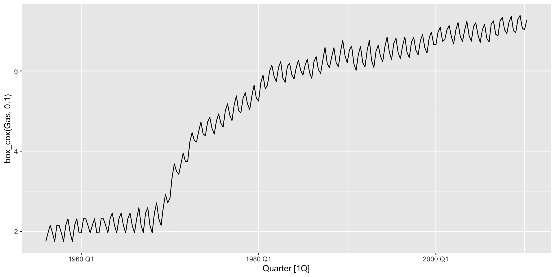
• So in the case of a Box-Cox transformation, \(\lambda\) should be chosen to make the size of the seasonal variation relatively constant across the whole series.

Mathematical transformations: Australian gas production

• Recall the time series of Australian gas production showed seasonality:

aus_production |>
  autoplot(Gas)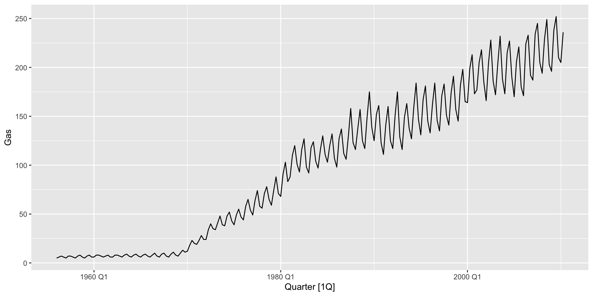

Mathematical transformations: Australian gas production

• Note that the variance of the seasonal trend is increasing over time.
• Try to smooth it out with a Box-Cox transformation. You can use autoplot(box_cox(Gas, lambda)) to do it automatically if you supply a lambda value.

Australian gas production: lambda = 0

aus_production |>
  autoplot(box_cox(Gas, 0))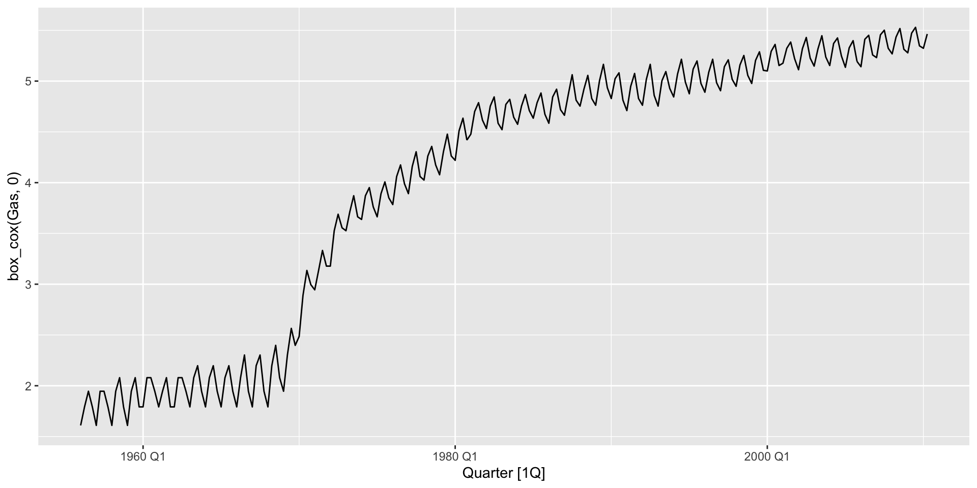

Australian gas production: lambda = 1

aus_production |>
  autoplot(box_cox(Gas, 1))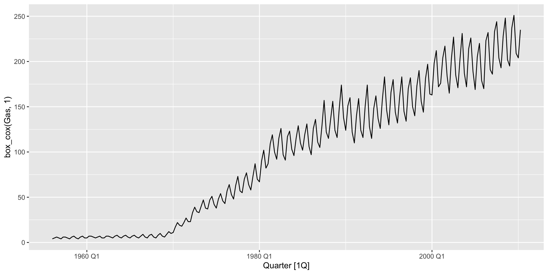

Australian gas production: lambda = 0.1

aus_production |>
  autoplot(box_cox(Gas, 0.1))