# A tsibble: 6 x 6 [1Q]
  Quarter Consumption Income Production Savings Unemployment
    <qtr>       <dbl>  <dbl>      <dbl>   <dbl>        <dbl>
1 1970 Q1       0.619  1.04      -2.45     5.30        0.9
2 1970 Q2       0.452  1.23      -0.551    7.79        0.5
3 1970 Q3       0.873  1.59      -0.359    7.40        0.5
4 1970 Q4      -0.272 -0.240     -2.19     1.17        0.700
5 1971 Q1       1.90   1.98       1.91     3.54       -0.100
6 1971 Q2 0.915 1.45 0.902 5.87 -0.100Time series regression in R
BUS 323 Forecasting and Risk Analysis
Getting set up
- We’ll work with the
us_changedataset today.
head(us_change)Plotting multiple series on a time plot
autoplotplots a single series across time.- We want to plot consumption and income change on one plot.
- To plot two, we’ll have to transform the data such that both series correspond to one variable. We can use
pivot_longer()to do so.
us_change |>
  pivot_longer(c(Consumption, Income), names_to="Series")
Plotting multiple series on a time plot
- Great, now we can autoplot
value
us_change |>
  pivot_longer(c(Consumption, Income), names_to="Series") |>
    autoplot(value) +
      labs(y = "% change")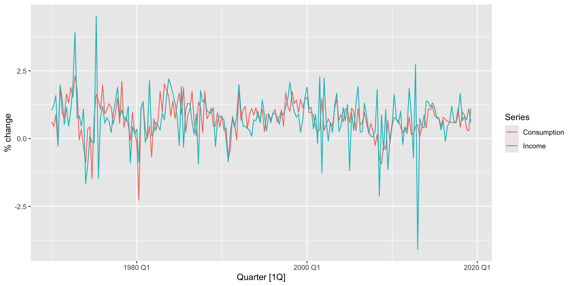
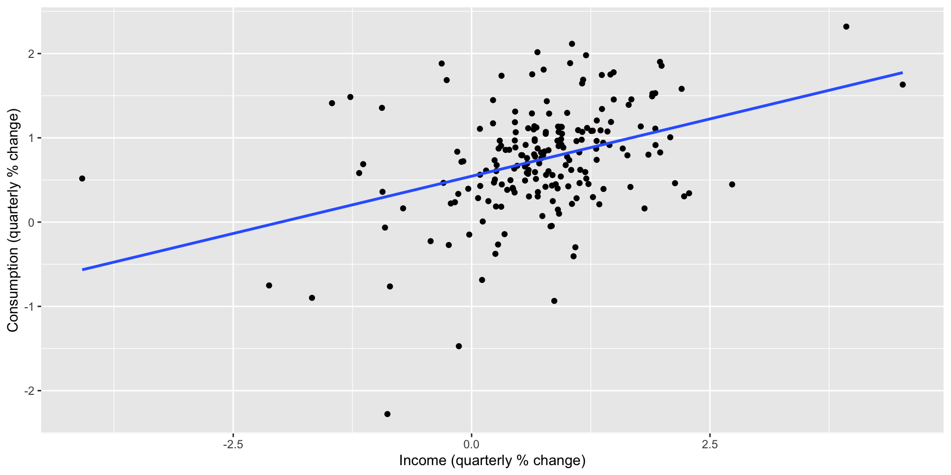
Plotting a line of best fit
- Adding a regression line to a scatterplot is simple with
geom_smoothand themethod = "lm"option:
us_change |>
  ggplot(aes(x = Income, y = Consumption)) +
  labs(y = "Consumption (quarterly % change)",
        x = "Income (quarterly % change)") +
  geom_point() +
  geom_smooth(method = "lm", se = FALSE)
Plotting a line of best fit
Estimating a regression function
- Suppose we want to estimate the following regression fucntion: \(y_{t} = \beta_{0} + \beta_{1} x_{t} + \epsilon_{t}\).
- Use
TSLM()to do so:
us_change |>
  model(TSLM(Consumption ~ Income)) |>
report()- Use
TSLM()instead oflm()because it has time series-friendly options built in.
Regression results
Series: Consumption
Model: TSLM

Residuals:
     Min       1Q   Median       3Q      Max
-2.58236 -0.27777  0.01862  0.32330  1.42229

Coefficients:
            Estimate Std. Error t value Pr(>|t|)
(Intercept)  0.54454    0.05403  10.079  < 2e-16 ***
Income       0.27183    0.04673   5.817  2.4e-08 ***
---
Signif. codes:  0 '***' 0.001 '**' 0.01 '*' 0.05 '.' 0.1 ' ' 1

Residual standard error: 0.5905 on 196 degrees of freedom
Multiple R-squared: 0.1472, Adjusted R-squared: 0.1429
F-statistic: 33.84 on 1 and 196 DF, p-value: 2.4022e-08
Multiple linear regression
- Regression with more than one regressor is called multiple regression: \(y_{t} = \beta_{0} + \beta_{1} x_{1,t} + \beta_{2} x_{2,t} + ... + \beta_{k} x_{k,t} + \epsilon_{t}\)
- Coefficients reflect conditional marginal effects
Multiple regression
- Pick a few variables in
us_changeto include in a multiple regression againstConsumption.
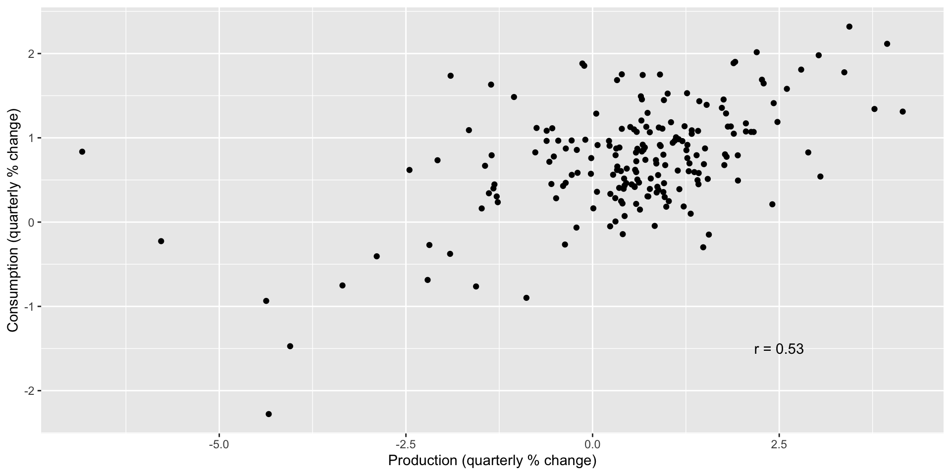
Consumption/production
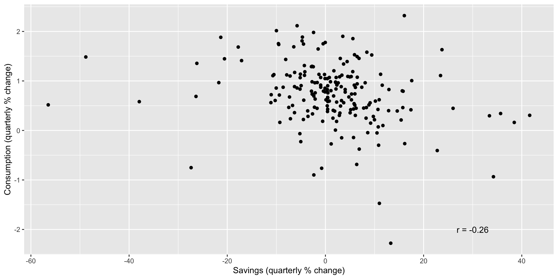
Consumption/savings
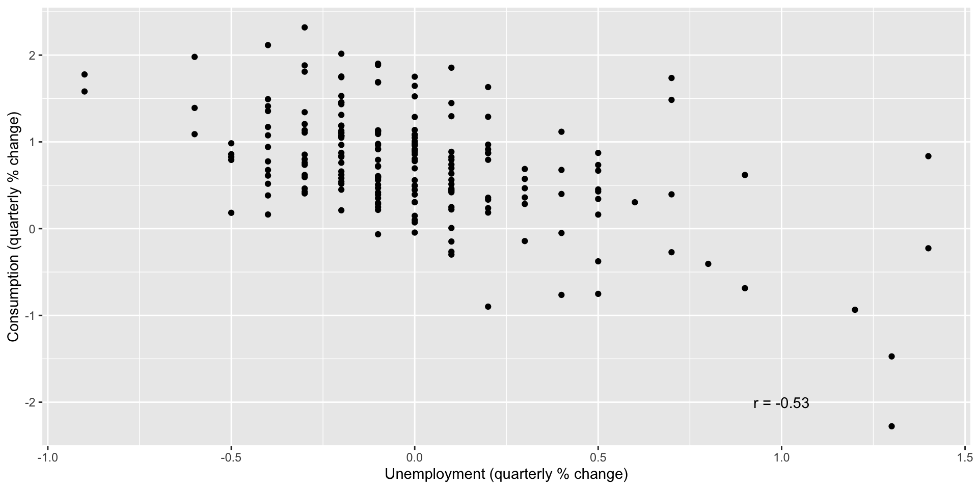
Consumption/unemployment
Multiple regression model
mr_c <- us_change |>
  model(TSLM(Consumption ~ Income + Production + Unemployment))
report(mr_c)
Multiple regression results
Series: Consumption
Model: TSLM

Residuals:
       Min         1Q     Median         3Q        Max
-1.5973206 -0.3317848 -0.0004972  0.2948522  1.6881414

Coefficients:
             Estimate Std. Error t value Pr(>|t|)
(Intercept)   0.55973    0.04915  11.389  < 2e-16 ***
Income        0.18044    0.04175   4.322 2.47e-05 ***
Production    0.10227    0.03756   2.722  0.00707 **
Unemployment -0.49026    0.15376  -3.188  0.00167 **
---
Signif. codes:  0 '***' 0.001 '**' 0.01 '*' 0.05 '.' 0.1 ' ' 1

Residual standard error: 0.508 on 194 degrees of freedom
Multiple R-squared: 0.3755, Adjusted R-squared: 0.3658
F-statistic: 38.88 on 3 and 194 DF, p-value: < 2.22e-16
Fitted values
- Estimating the regression allows us to obtain fitted (predicted) values for \(y\): \(\hat{y}_{t} = \hat{\beta}_{0} + \hat{\beta}_{1} x_{1,t} + \hat{\beta}_{2} x_{2,t} + ... + \hat{\beta}_{k} x_{k,t} + \epsilon_{t}\)
- Note these are predictions for the actual observed values, not forecasts.
Accessing fitted values
- With a
tslmobject, useaugment()to access fitted values:
augment(mr_c)# A tsibble: 198 x 6 [1Q]
# Key: .model [1]
.model Quarter Consumption .fitted .resid .innov
<chr> <qtr> <dbl> <dbl> <dbl> <dbl>
1 TSLM(Consumption ~ Income + Prod… 1970 Q1 0.619 0.0562 0.562 0.562
2 TSLM(Consumption ~ Income + Prod… 1970 Q2 0.452 0.479 -0.0274 -0.0274
3 TSLM(Consumption ~ Income + Prod… 1970 Q3 0.873 0.564 0.309 0.309
4 TSLM(Consumption ~ Income + Prod… 1970 Q4 -0.272 -0.0502 -0.222 -0.222
5 TSLM(Consumption ~ Income + Prod… 1971 Q1 1.90 1.16 0.741 0.741
6 TSLM(Consumption ~ Income + Prod… 1971 Q2 0.915 0.962 -0.0470 -0.0470
7 TSLM(Consumption ~ Income + Prod… 1971 Q3 0.794 0.636 0.158 0.158
8 TSLM(Consumption ~ Income + Prod… 1971 Q4 1.65 1.00 0.642 0.642
9 TSLM(Consumption ~ Income + Prod… 1972 Q1 1.31 1.17 0.146 0.146
10 TSLM(Consumption ~ Income + Prod… 1972 Q2 1.89 0.988 0.897 0.897
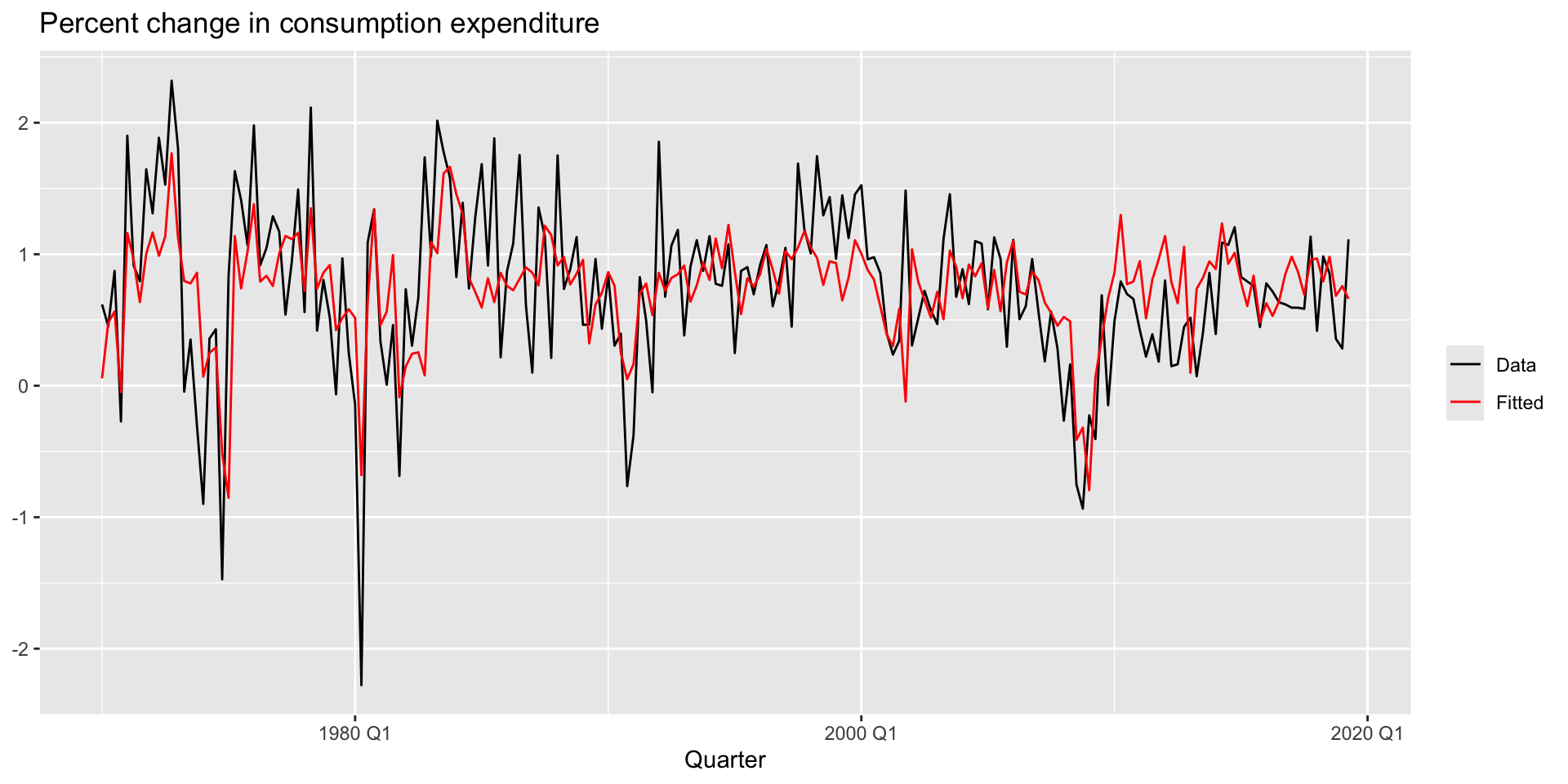
# ℹ 188 more rowsPlotting fitted values
- Let’s see how well our predicted values line up with reality.
augment(mr_c) |>
  ggplot(aes(x = Quarter)) +
  geom_line(aes(y = Consumption, colour = "Data")) +
  geom_line(aes(y = .fitted, colour = "Fitted")) +
  labs(y = NULL,
  title = "Percent change in consumption expenditure") +
  scale_colour_manual(values=c(Data="black",Fitted="red")) +
  guides(colour = guide_legend(title = NULL))
Plotting fitted values
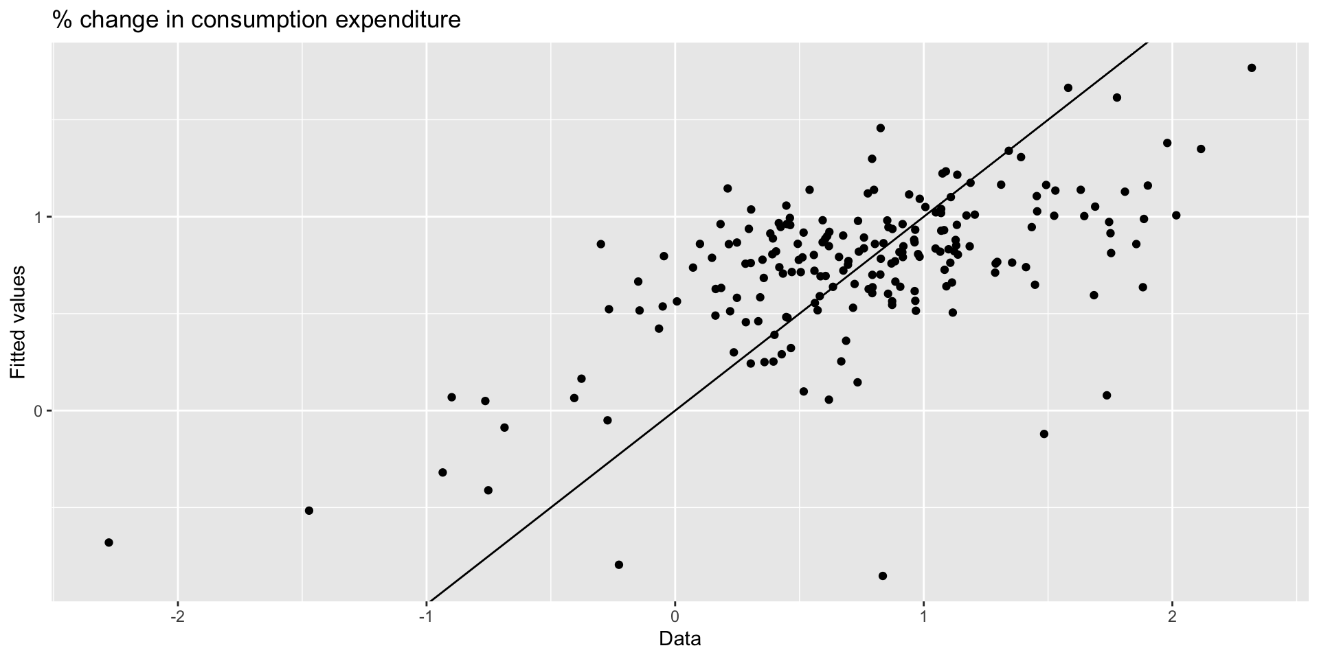
Plotting fitted values: scatter
- We could scatter \(y\) against \(\hat{y}\):
augment(mr_c) |>
  ggplot(aes(x = Consumption, y = .fitted)) +
  geom_point() +
  labs(x = "Data",
  y = "Fitted values",
  title = "% change in consumption expenditure") +
  geom_abline(intercept = 0, slope = 1)
Plotting fitted values: scatter
Goodness-of-fit
- The coefficient of determination, \(R^{2}\) is a good summary measure of how well your model fits the data:
\(R^{2} = \frac{\sum(\hat{y}_{t} - \bar{y})^{2}}{\sum(y_{t} - \bar{y})^{2}}\)
- It gives the proportion of variation in \(y\) explained by \(\hat{y}\).
- Note \(R^{2}\) never decreases when adding predictors. Not necessarily a good metric for evaluating a forecast model.
- \(R^{2}\) of above model is 0.3755.