| Year | Observation |
|---|---|
| 2015 | 123 |
| 2016 | 39 |
| 2017 | 78 |
| 2018 | 52 |
| 2019 | 110 |
Time series graphics
BUS 323 Forecasting and Risk Analysis
The pipe operator
- The pipe operator (
%>%, or|>) allows you to write your code in a more stepwise fashion. - Instead of:
mutate(filter(data, x > 5),
y = y * 2)- You can write:
data %>%
  filter(x > 5) %>%
  mutate(y = y * 2)
Data manipulation functions: filter
filter(): selects rows based on conditions.- e.g.
data |> filter(x > 5)will return the observations within object data that match the filter condition.
Data manipulation functions: mutate
mutate(): adds or transforms columns.- e.g.
data |> mutate(y = y*2)will return data with the observations in column y doubled.
Data manipulation functions: select
select(): chooses specific columns.- e.g.
data |> select(x)will return only the x column of data.
Data manipulation functions: arrange
arrange(): sorts rows by column values.- e.g.
data |> arrange(desc(x))will return data with rows sorted by x in descending order.
Data manipulation functions: summarise and group_by
summarise(): aggregates datagroup_by(): groups data by a column value- e.g.
data |>
group_by(x) |>
summarise(average_y = mean(y))
will return the mean of y conditional on x.
Time series graphics in R
- Load up RStudio
- Packages tab -> Install -> fpp3
- Check “install dependencies”
- Load the fpp3 package by running
library(fpp3)in your session.
tsibble objects
- tsibble objects format time series in a tidy way.
- Suppose we have the following:
tsibble objects
- We can turn it into a tsibble object with the following command:
y <- tsibble(
  Year = 2015:2019,
  Observation = c(123, 39, 78, 52, 110),
  index = Year
)
Working with tsibble objects
- Once you have a tsibble, working with it is simple. Run:
PBS
# A tsibble: 67,596 x 9 [1M]
# Key:       Concession, Type, ATC1, ATC2 [336]
      Month Concession   Type      ATC1  ATC1_desc ATC2  ATC2_desc Scripts  Cost
      <mth> <chr>        <chr>     <chr> <chr>     <chr> <chr>       <dbl> <dbl>
 1 1991 Jul Concessional Co-payme… A     Alimenta… A01   STOMATOL…   18228 67877
 2 1991 Aug Concessional Co-payme… A     Alimenta… A01   STOMATOL…   15327 57011
 3 1991 Sep Concessional Co-payme… A     Alimenta… A01   STOMATOL…   14775 55020
 4 1991 Oct Concessional Co-payme… A     Alimenta… A01   STOMATOL…   15380 57222
 5 1991 Nov Concessional Co-payme… A     Alimenta… A01   STOMATOL…   14371 52120
 6 1991 Dec Concessional Co-payme… A     Alimenta… A01   STOMATOL…   15028 54299
 7 1992 Jan Concessional Co-payme… A     Alimenta… A01   STOMATOL…   11040 39753
 8 1992 Feb Concessional Co-payme… A     Alimenta… A01   STOMATOL…   15165 54405
 9 1992 Mar Concessional Co-payme… A     Alimenta… A01   STOMATOL…   16898 61108
10 1992 Apr Concessional Co-payme… A     Alimenta… A01   STOMATOL…   18141 65356
# ℹ 67,586 more rows
Working with tsibble objects
- Suppose we are interested in A10 scripts specifically:
PBS |>
  filter(ATC2 == "A10")
# A tsibble: 816 x 9 [1M]
# Key: Concession, Type, ATC1, ATC2 [4]
Month Concession Type ATC1 ATC1_desc ATC2 ATC2_desc Scripts Cost
<mth> <chr> <chr> <chr> <chr> <chr> <chr> <dbl> <dbl>
1 1991 Jul Concessional Co-paym… A Alimenta… A10 ANTIDIAB… 89733 2.09e6
2 1991 Aug Concessional Co-paym… A Alimenta… A10 ANTIDIAB… 77101 1.80e6
3 1991 Sep Concessional Co-paym… A Alimenta… A10 ANTIDIAB… 76255 1.78e6
4 1991 Oct Concessional Co-paym… A Alimenta… A10 ANTIDIAB… 78681 1.85e6
5 1991 Nov Concessional Co-paym… A Alimenta… A10 ANTIDIAB… 70554 1.69e6
6 1991 Dec Concessional Co-paym… A Alimenta… A10 ANTIDIAB… 75814 1.84e6
7 1992 Jan Concessional Co-paym… A Alimenta… A10 ANTIDIAB… 64186 1.56e6
8 1992 Feb Concessional Co-paym… A Alimenta… A10 ANTIDIAB… 75899 1.73e6
9 1992 Mar Concessional Co-paym… A Alimenta… A10 ANTIDIAB… 89445 2.05e6
10 1992 Apr Concessional Co-paym… A Alimenta… A10 ANTIDIAB… 97315 2.23e6
# ℹ 806 more rowsWorking with tsibble objects
- And suppose we only want to use the variables Month, Concession, Type, and Cost:
PBS |>
  filter(ATC2 == "A10") |>
  select(Month, Concession, Type, Cost)
# A tsibble: 816 x 4 [1M]
# Key: Concession, Type [4]
Month Concession Type Cost
<mth> <chr> <chr> <dbl>
1 1991 Jul Concessional Co-payments 2092878
2 1991 Aug Concessional Co-payments 1795733
3 1991 Sep Concessional Co-payments 1777231
4 1991 Oct Concessional Co-payments 1848507
5 1991 Nov Concessional Co-payments 1686458
6 1991 Dec Concessional Co-payments 1843079
7 1992 Jan Concessional Co-payments 1564702
8 1992 Feb Concessional Co-payments 1732508
9 1992 Mar Concessional Co-payments 2046102
10 1992 Apr Concessional Co-payments 2225977
# ℹ 806 more rowsWorking with tsibble objects
- Suppose further we are only interested in total cost regardless of concession or type:
PBS |>
  filter(ATC2 == "A10") |>
  select(Month, Concession, Type, Cost) |>
  summarise(TotalC = sum(Cost))
# A tsibble: 204 x 2 [1M]
Month TotalC
<mth> <dbl>
1 1991 Jul 3526591
2 1991 Aug 3180891
3 1991 Sep 3252221
4 1991 Oct 3611003
5 1991 Nov 3565869
6 1991 Dec 4306371
7 1992 Jan 5088335
8 1992 Feb 2814520
9 1992 Mar 2985811
10 1992 Apr 3204780
# ℹ 194 more rowsWorking with tsibble objects
- You can make new variables using
mutate(). Let’s convertTotalCto millions of dollars:
PBS |>
  filter(ATC2 == "A10") |>
  select(Month, Concession, Type, Cost) |>
  summarise(TotalC = sum(Cost)) |>
  mutate(Cost = TotalC/1e6)
# A tsibble: 204 x 3 [1M]
Month TotalC Cost
<mth> <dbl> <dbl>
1 1991 Jul 3526591 3.53
2 1991 Aug 3180891 3.18
3 1991 Sep 3252221 3.25
4 1991 Oct 3611003 3.61
5 1991 Nov 3565869 3.57
6 1991 Dec 4306371 4.31
7 1992 Jan 5088335 5.09
8 1992 Feb 2814520 2.81
9 1992 Mar 2985811 2.99
10 1992 Apr 3204780 3.20
# ℹ 194 more rowsWorking with tsibble objects
- To save something for future use, use the assignment operator
<-:
a10 <- PBS |>
  filter(ATC2 == "A10") |>
  select(Month, Concession, Type, Cost) |>
  summarise(TotalC = sum(Cost)) |>
  mutate(Cost = TotalC/1e6)
Time plots
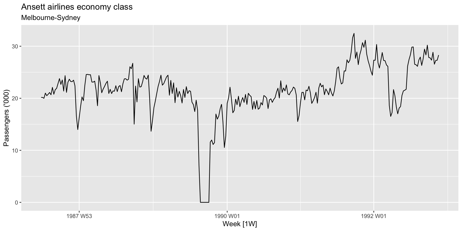
- Plot thousands of economy passengers flying between Melbourne (MEL) and Sydney (SYD) airports from the
ansettdataset infpp3using theautoplot()command:
Time plots
- Plot thousands of economy passengers flying between Melbourne (MEL) and Sydney (SYD) airports from the
ansettdataset infpp3using theautoplot()command:
melsyd_economy <- ansett |>
  filter(Airports == "MEL-SYD", Class == "Economy") |>
  mutate(Passengers = Passengers/1000)
autoplot(melsyd_economy, Passengers) +
  labs(title = "Ansett airlines economy class",
       subtitle = "Melbourne-Sydney",
       y = "Passengers ('000)")
Time plots
- Plot thousands of economy passengers flying between Melbourne (MEL) and Sydney (SYD) airports from the
ansettdataset infpp3using theautoplot()command:
Time series patterns
- Cyclicality: occurs when the data exhibit rises and falls of regular but not fixed frequency. If a fluctuation occurs with a fixed frequency and is related to the calendar, it’s seasonal.
- Exercise time
Exercise: electricity
aus_production |>
  filter(year(Quarter) >= 1980) |>
  autoplot(Electricity) +
  labs(y = "GWh", title = "Australian electricity production")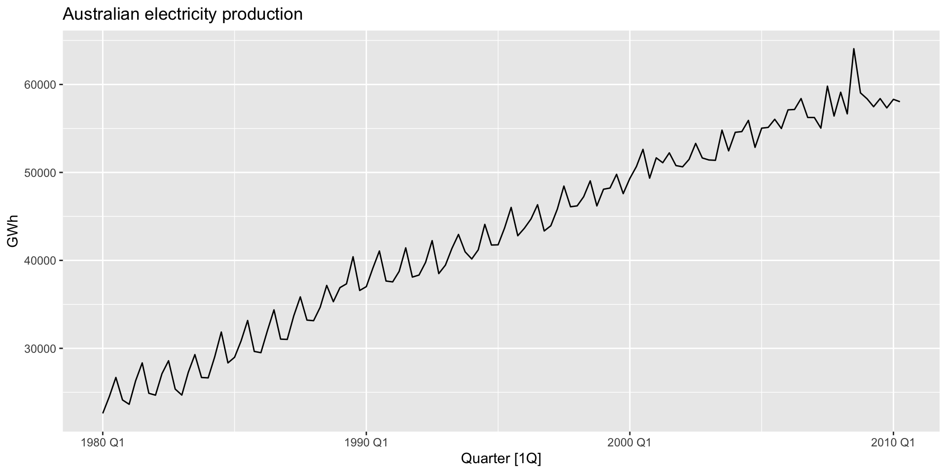
Exercise: bricks
aus_production |>
  autoplot(Bricks) +
  labs(y = "million units", title = "Australian clay brick production")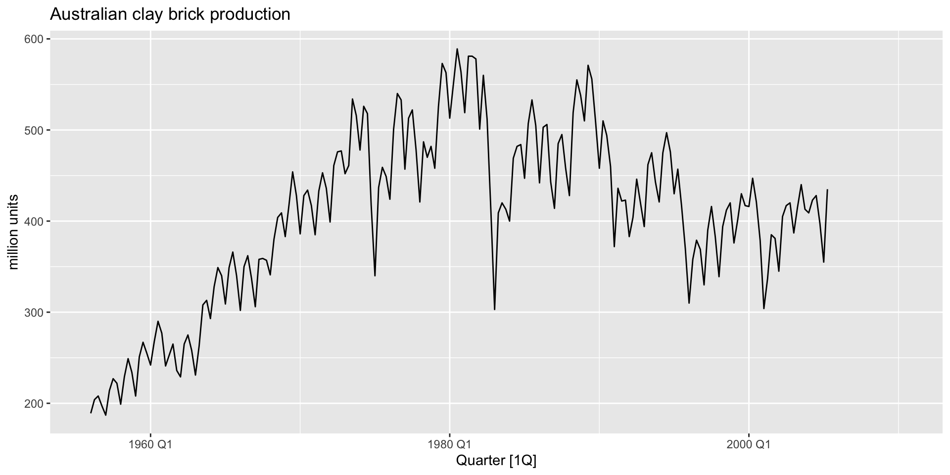
Exercise: retail employment
us_employment |>
  filter(Title == "Retail Trade", year(Month) >= 1980) |>
  autoplot(Employed / 1000) +
  labs(y = "Million people", title = "Retail employment, USA")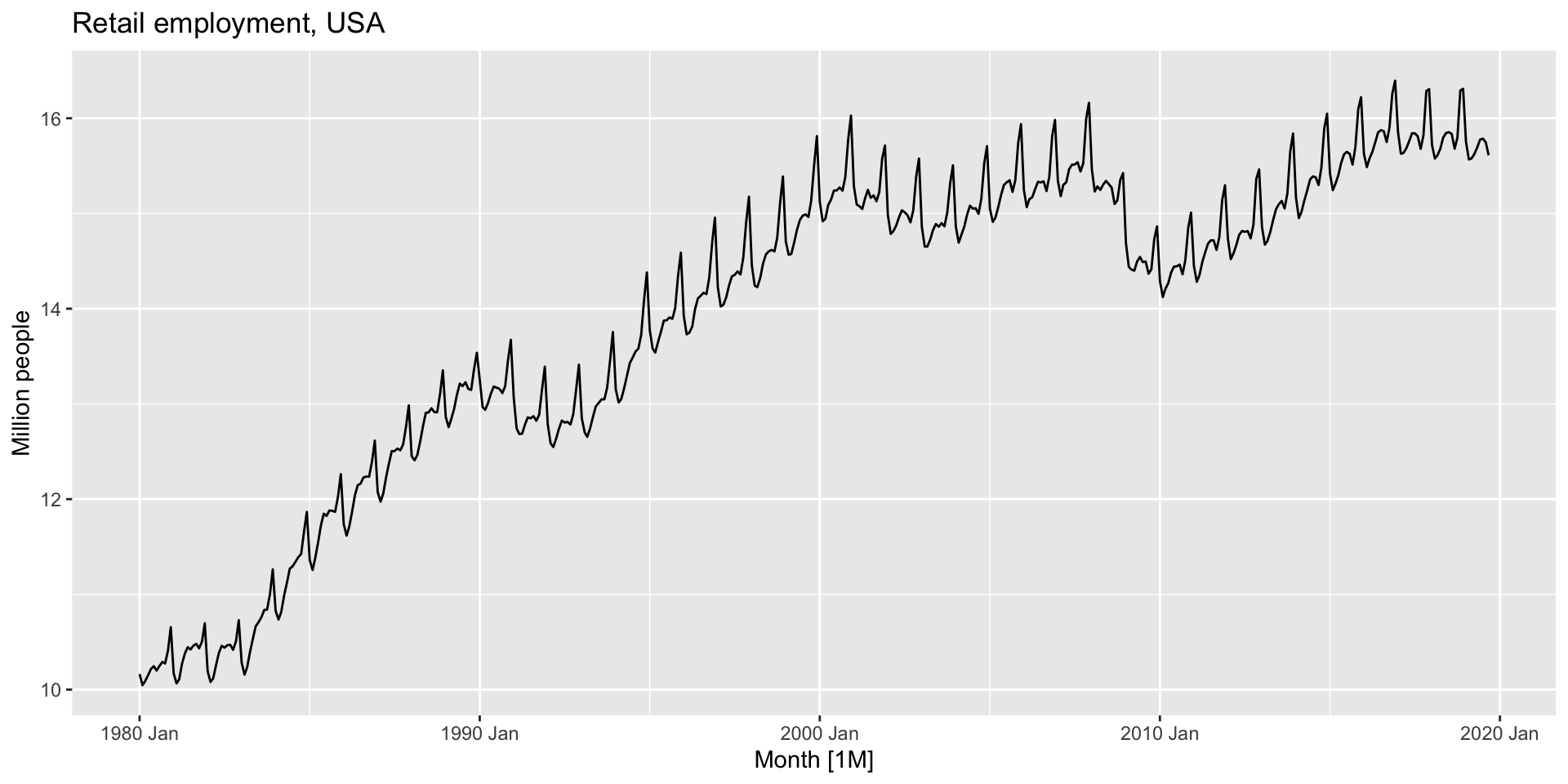
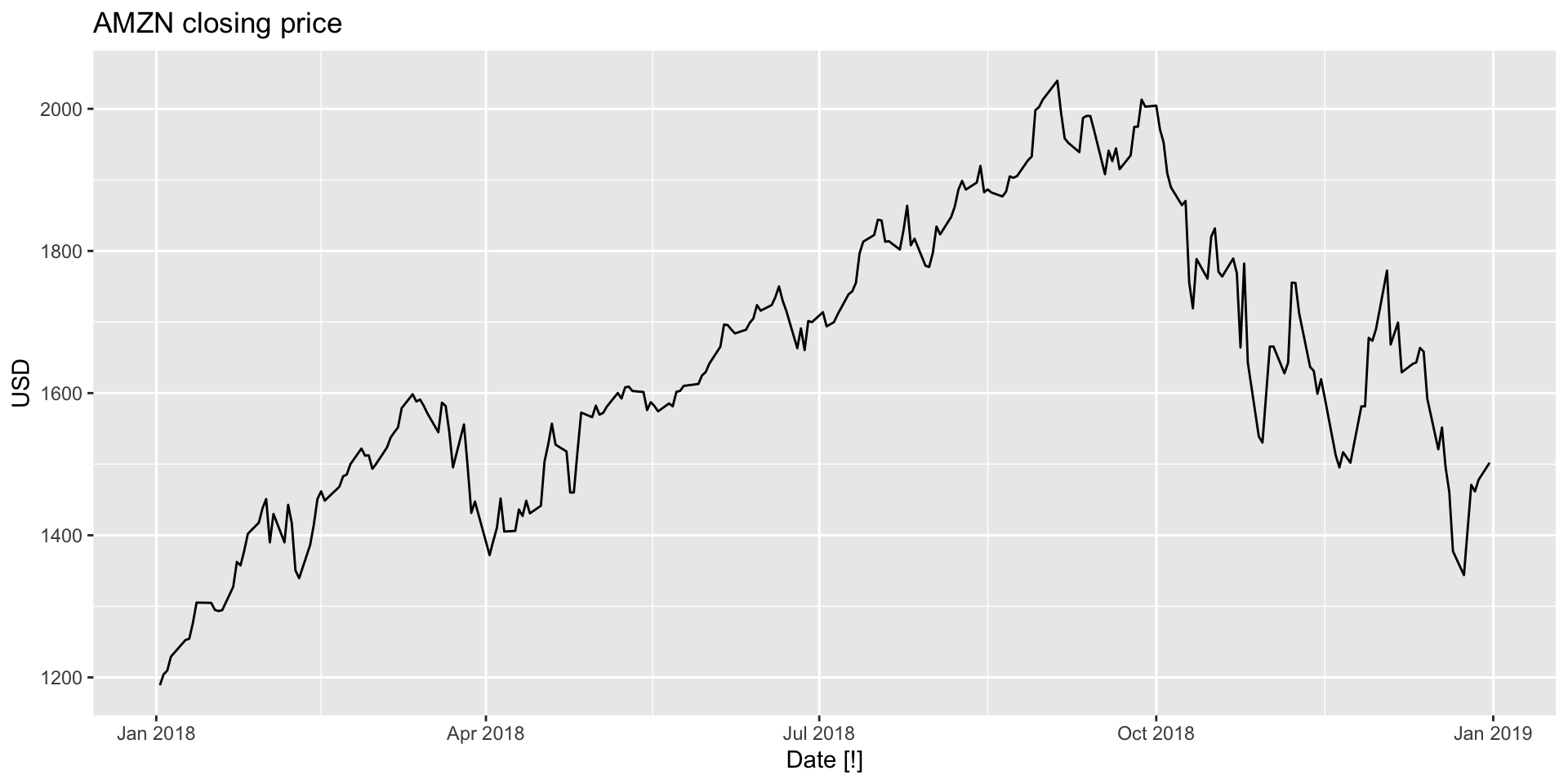
Exercise: AMZN
gafa_stock |>
  filter(Symbol == "AMZN", year(Date) >= 2018) |>
  autoplot(Close) +
  labs(y = "USD", title = "AMZN closing price")