Seasonal ARIMA models

BUS 323 Forecasting and Risk Analysis

Seasonal ARIMA models

Non-seasonal component defined by \((p,d,q)\).
Seasonal component defined by \((P,D,Q)_{m}\).
- \(m\): seasonal period *e.g. ARIMA(1,1,1)(1,1,1)\(_{4}\):
- AR(1), MA(1), first differencing, quarterly data
  
  \[ y_{t}' = c + \phi_{1} y_{t-1}' + \Phi_{1} y_{t-4}' + \theta_{1} \epsilon_{t-1} + \Theta_{1} \epsilon_{t-4}' + \epsilon_{t} \]

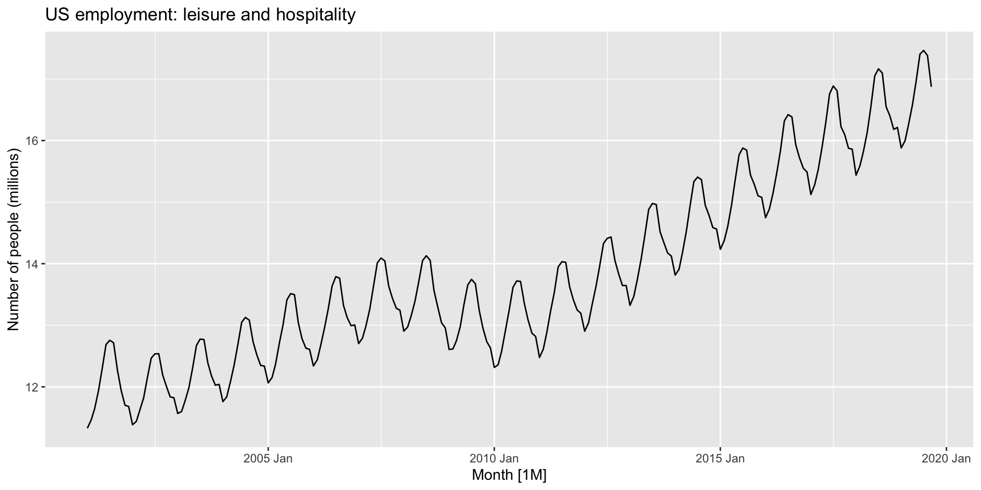
Example: seasonal employment

Monthly leisure and hospitality employment in the US
Use us_employment from fpp3.
Filter based on Title=="Leisure and Hospitality" and year(Month) > 2000

Example: setup

library(fpp3)
leisure <- us_employment |>
  filter(Title == "Leisure and Hospitality",
         year(Month) > 2000) |>
  mutate(Employed = Employed/1000) |>
  select(Month, Employed)
autoplot(leisure, Employed) +
  labs(title = "US employment: leisure and hospitality",
       y="Number of people (millions)")

Example: time plot

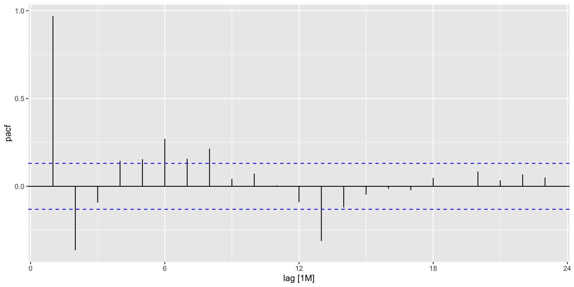
Partial autocorrelation plots

Measure correlation between \(y_{t}\) and \(y_{t-k}\) after removing the effects of lags 1, 2, 3, …, \(k-1\).
\(\alpha_{k} = \phi_{k}\) in an AR(\(k\)) model.

PACF plots in R

leisure |>
  PACF(Employed) |>
  autoplot()

PACF plots in R

Another option: use gg_tsdisplay() with option plot_type = "partial"

PACF plots: interpretation

ARIMA(\(p,d,0\)) if with differenced data:
- ACF exponentially decaying or sinusoidal.
- Significant spike at lag \(p\) in PACF but none beyond lag \(p\).
ARIMA(\(0,d,q\)) if with differenced data:
- PACF exponentially decaying or sinusooidal.
- Significant spike at lag \(q\) in ACF but none beyond lag \(q\).

Example: towards an ARIMA

The data are non-stationary. What to do?
First difference?

leisure |>
  gg_tsdisplay(difference(Employed, 12),
               plot_type='partial', lag=36) +
  labs(title="Seasonally differenced", y="")

Example: first difference plots

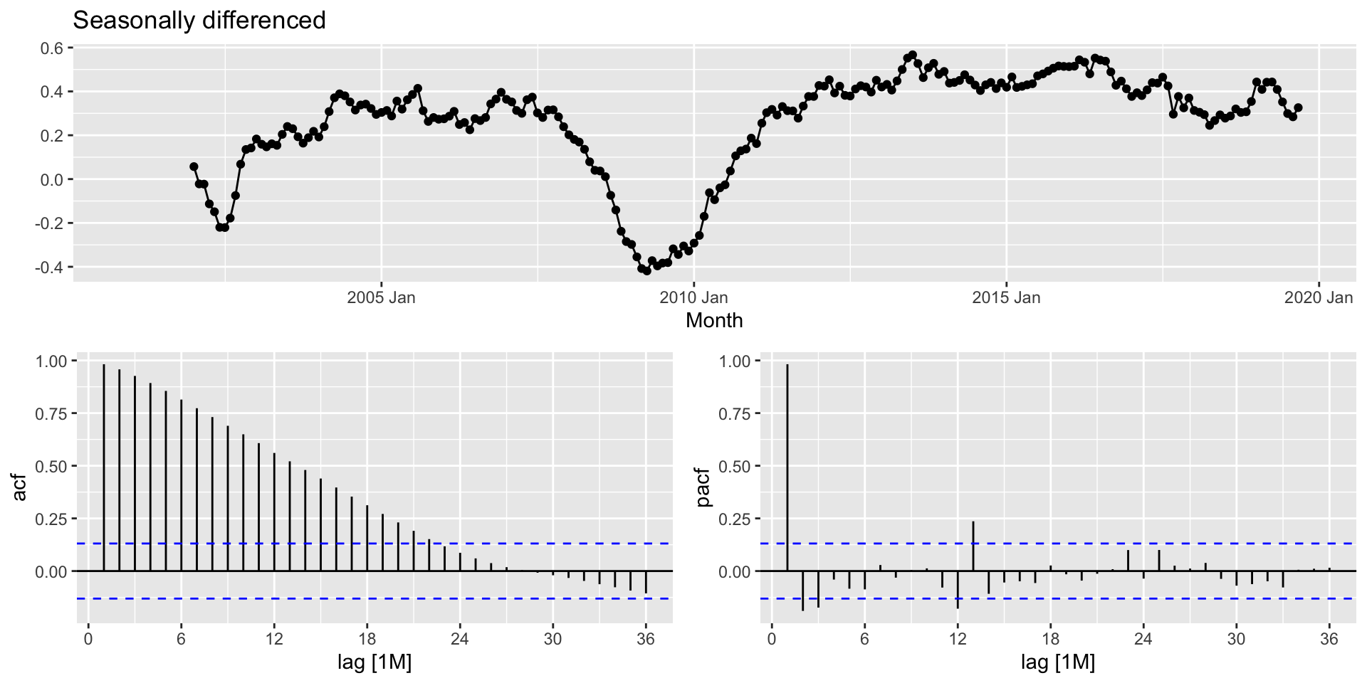
Example: towards an ARIMA, again

Still non-stationary. Now what?
Second difference?

leisure |>
  gg_tsdisplay(difference(Employed, 12) |> difference(),
               plot_type='partial', lag=36) +
  labs(title = "Double differenced", y="")

Example: double-difference plots

Example: Model selection

ACF spike at lag 2 \(\rightarrow\) non-seasonal MA(2).
ACF spike at lag 12 \(\rightarrow\) seasonal MA(1).
We need:
- First difference
- Seasonal difference
- Non-seasonal MA(2)
- Seasonal MA(1)
ARIMA(0,1,2)(0,1,1)\(_{12}\)

Example: Model selection

Or maybe…
- PACF spike at lag 2 \(\rightarrow\) non-seasonal AR(2)
- PACF spike at lag 12 \(\rightarrow\) seasonal MA(1)
We need:
- First difference
- Seasonal difference
- Non-seasonal AR(2)
- Seasonal MA(1)
ARIMA(2,1,0)(0,1,1)\(_{12}\)

Example: estimation

Let’s estimate both
Also allow for automatic selection.

fit <- leisure |>
  model(
    arima012011 = ARIMA(Employed ~ pdq(0,1,2) + PDQ(0,1,1)),
    arima210011 = ARIMA(Employed ~ pdq(2,1,0) + PDQ(0,1,1)),
    auto = ARIMA(Employed, stepwise = FALSE, approx = FALSE)
  )
fit

# A mable: 1 x 3
                arima012011               arima210011                      auto
                    <model>                   <model>                   <model>
1 <ARIMA(0,1,2)(0,1,1)[12]> <ARIMA(2,1,0)(0,1,1)[12]> <ARIMA(2,1,0)(1,1,1)[12]>

Example: estimation

In ARIMA() options:
- stepwise=FALSE: use ``TRUE``` by default
- approx=FALSE: use this by default

fit <- leisure |>
  model(
    arima012011 = ARIMA(Employed ~ pdq(0,1,2) + PDQ(0,1,1)),
    arima210011 = ARIMA(Employed ~ pdq(2,1,0) + PDQ(0,1,1)),
    auto = ARIMA(Employed, stepwise = FALSE, approx = FALSE)
  )
glance(fit)

# A tibble: 3 × 8
  .model       sigma2 log_lik   AIC  AICc   BIC ar_roots   ma_roots  
  <chr>         <dbl>   <dbl> <dbl> <dbl> <dbl> <list>     <list>    
1 arima012011 0.00146    391. -775. -775. -761. <cpl [0]>  <cpl [14]>
2 arima210011 0.00145    392. -776. -776. -763. <cpl [2]>  <cpl [12]>
3 auto        0.00142    395. -780. -780. -763. <cpl [14]> <cpl [12]>

Example: evaluation

Let’s look at the residuals from our best model:

fit |>
  select(auto) |>
  gg_tsresiduals(lag=36)

Example: evaluation

Let’s look at the residuals from our best model:

Example: portmanteau test

One spike in the ACF is still consistent with white noise
Let’s do a Ljung-Box test just for fun:

augment(fit) |>
  filter(.model == "auto") |>
  features(.innov, ljung_box, lag=24, dof=4)

# A tibble: 1 × 3
  .model lb_stat lb_pvalue
  <chr>    <dbl>     <dbl>
1 auto      16.6     0.680

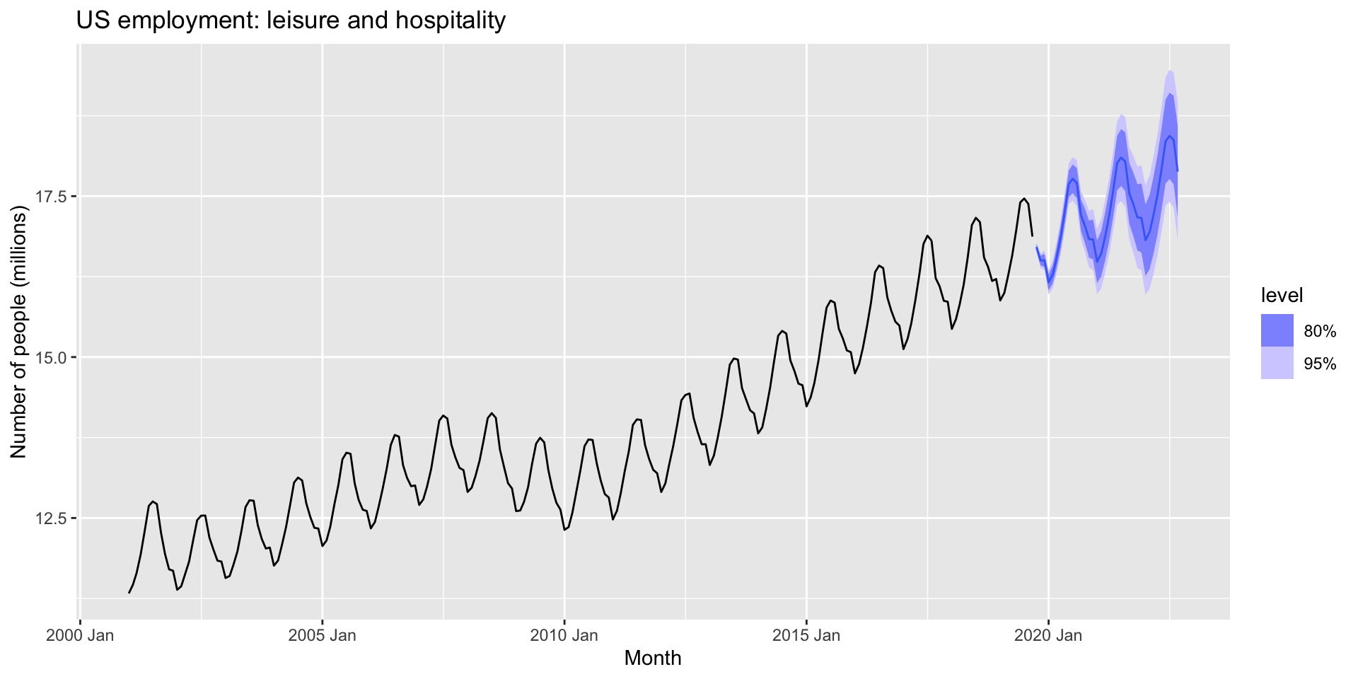
Example: forecast

Let’s use our model to make a forecast.

forecast(fit, h=36) |>
  filter(.model=='auto') |>
  autoplot(leisure) +
  labs(title = "US employment: leisure and hospitality",
       y="Number of people (millions)")

Example: forecast

Let’s use our model to make a forecast.

Example 2: drug sales

Forecast monthly corticosteroid drug sales in Australia
Use PBS dataset
Filter based on ATC2=="H02")
Note you want total monthly sales for this type of drug.
Find a suitable ARIMA model, check that its residuals follow a white noise process, forecast 24 months into the future.