ARIMA I

BUS 323 Forecasting and Risk Analysis

Unit root tests

Test whether a series has a unit root.
- A series has a unit root if it is integrated of order 1.
- That is, if it needs to be differenced to be stationary.
Kwiatkowski-Phillips-Schmidt-Shin (KPSS) test and Augmented Dickey-Fuller (ADF) test most common.

Implementation

Use unitroot_kpss():

library(fpp3)
google_2015 <- gafa_stock |>
  filter(Symbol == "GOOG", year(Date) == 2015)

google_2015 |>
  features(Close, unitroot_kpss)

# A tibble: 1 × 3
  Symbol kpss_stat kpss_pvalue
  <chr>      <dbl>       <dbl>
1 GOOG        3.56        0.01

Interpretation

unitroot_kpss() reports the p-value associated with the KPSS test.
\(H_{0}\) of the KPSS test is that the data are stationary.
- p-value of above was 0.01 or less
- \(\rightarrow\) reject \(H_{0}\)
- \(\rightarrow\) data are non-stationary.
- Difference the data and re-apply test.

Trying again…

Apply unit root test to Close':

google_2015 |>
  mutate(diff_close = difference(Close)) |>
  features(diff_close, unitroot_kpss)

# A tibble: 1 × 3
  Symbol kpss_stat kpss_pvalue
  <chr>      <dbl>       <dbl>
1 GOOG      0.0989         0.1

How many differences?

Use unitroot_ndiffs() to find how mnay differences will be needed before the test detects a unit root.
- Use unitroot_nsdiffs() for seasonal data.
Try it on monthly Australian retail turnover (from aus_retail).

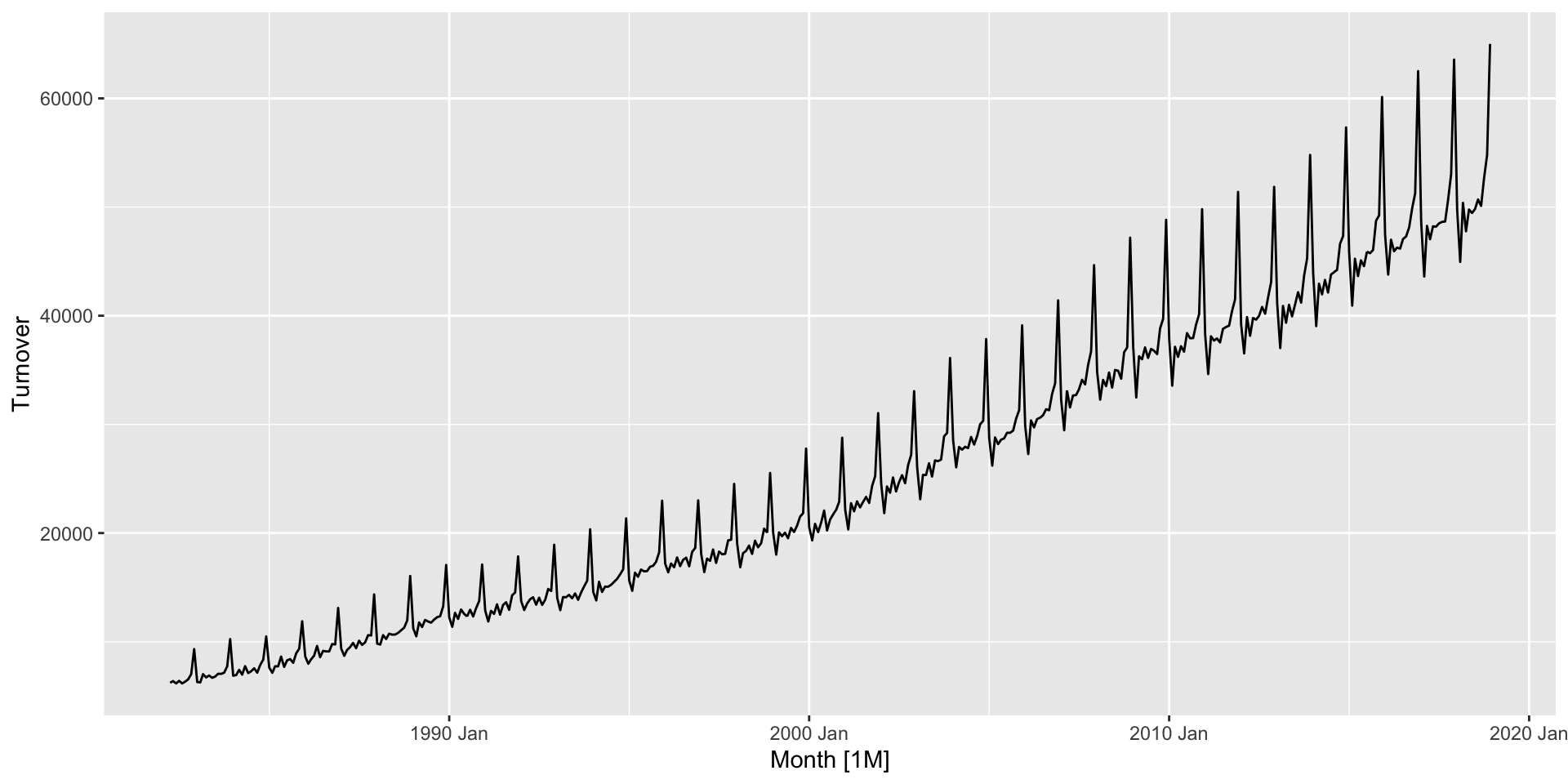
Example: Australian retail turnover

aus_total_retail <- aus_retail |>
  summarise(Turnover = sum(Turnover)) 
aus_total_retail |>
  autoplot(Turnover)

Example: Australian retail turnover

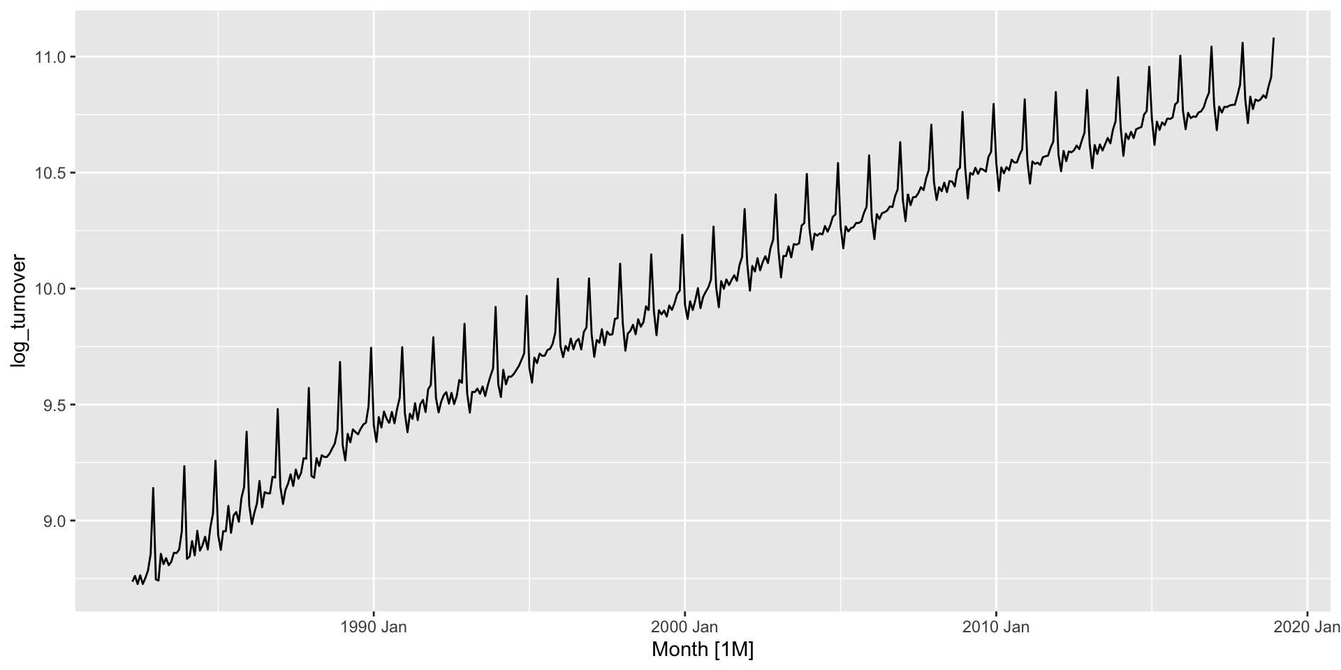
Let’s try to log it:

aus_total_retail |>
  mutate(log_turnover = log(Turnover)) |>
  autoplot(log_turnover)

Example: Australian retail turnover

Try using unitroot_nsdiffs():

aus_total_retail |>
  mutate(log_turnover = log(Turnover)) |>
  features(log_turnover, unitroot_nsdiffs)

# A tibble: 1 × 1
  nsdiffs
    <int>
1       1

Example: Australian retail turnover

Apply seasonal difference, then perform unit root test again:

aus_total_retail |>
  mutate(log_turnover = difference(log(Turnover), 12)) |>
  features(log_turnover, unitroot_ndiffs)

# A tibble: 1 × 1
  ndiffs
   <int>
1      1

Example: Australian retail turnover

The test suggests one more difference is needed:

Example: Australian retail turnover

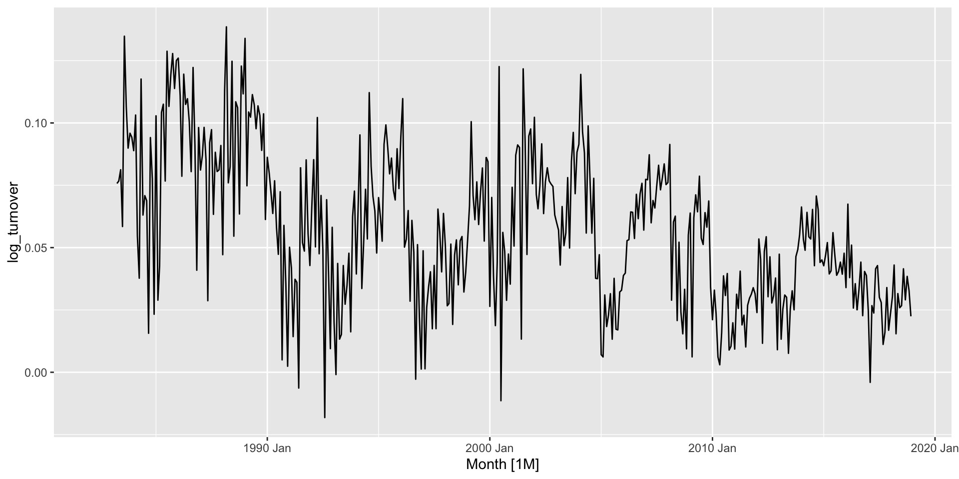
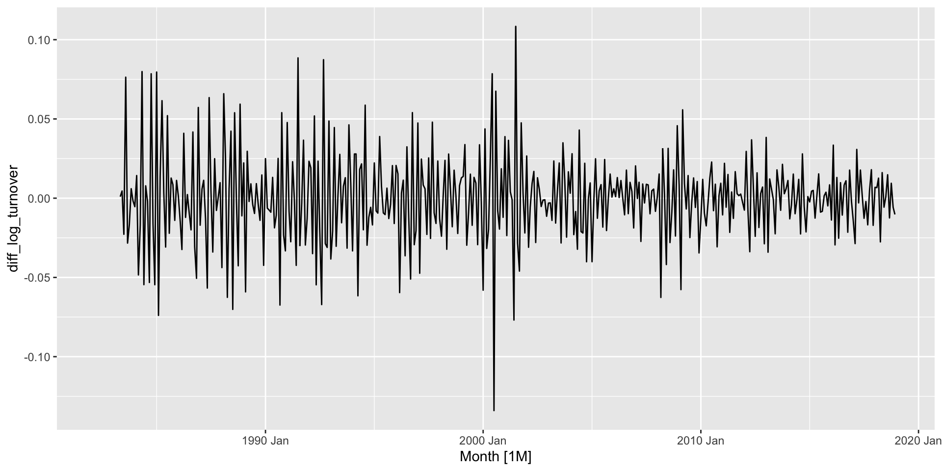
Difference the seasonally differenced data, then test again:

aus_total_retail |>
  mutate(diff_log_turnover = difference(difference(log(Turnover),12),1)) |>
  features(diff_log_turnover, unitroot_ndiffs)

# A tibble: 1 × 1
  ndiffs
   <int>
1      0

Example: Australian retail turnover

Autoregressive models

Forecast \(y_{t}\) based on past values of \(y\).
AR(\(p\)):

\[ y_{t} = c + \phi_{1} y_{t-1} + \phi_{2} y_{t-2} + ... + \phi_{p} y_{t-p} + \epsilon_{t} \]

Autoregressive models

For an AR(1) model:
- \(\phi_{1}=0\) and \(c=0\), \(y_{t}\) is white noise.
- \(\phi_{1} =1\) and \(c=0\), \(y_{t}\) is a random walk.
- \(\phi_{1}=1\) and \(c \neq 0\), \(y_{t}\) is a random walk with drift.
- \(\phi_{1} < 0\) results in \(y_{t}\) oscillating around its mean.

Autoregressive models

AR models perform best on stationary data.
Necessary constraints on parameters:
- For an AR(1): \(-1 < \phi_{1} < 1\).
- For an AR(2): \(-1 < \phi_{2} < 1\); \(\phi_{1} + \phi_{2} < 1\); \(\phi_{2} - \phi_{1} < 1\).

Implementation

Use ARIMA() (more later). Specify \(p\) in the first argument of the function.
e.g. let’s estimate an AR(2) based on the stationary series we found above:

ar_fit <- aus_total_retail |>
  mutate(diff_log_turnover = difference(difference(log(Turnover),12),1)) |>
  model(ar2 = ARIMA(diff_log_turnover ~ pdq(2,0,0)))
glance(ar_fit)

# A tibble: 1 × 8
  .model   sigma2 log_lik    AIC   AICc    BIC ar_roots   ma_roots 
  <chr>     <dbl>   <dbl>  <dbl>  <dbl>  <dbl> <list>     <list>   
1 ar2    0.000350   1089. -2168. -2168. -2148. <cpl [26]> <cpl [0]>

Exercise

Apply an AR(1) and AR(2) model to the stationary series derived last time. Which fits better? Try to plot the forecast and the data.