Time Series Regression: The Return

BUS 323 Forecasting and Risk Analysis

Selecting predictors

• Often many potential predictors
• For causal inference: theory
• For improved fit: a measure of accuracy
  • We’ll look at a few.

Adjusted \(R^{2}\)

• Additional regressors always increase \(R^{2}\).

  • Use adjusted \(R^{2}\) instead.

    \[ \bar{R}^{2} = 1 - (1 - R^{2}) \frac{T - 1}{T - k - 1} \]

  • \(T\): # of observations

  • \(k\): # of predictors

• Maximizing \(\bar{R}^{2}\) minimizes standard error.

Cross-validation

• Leave-one-out cross-validation
  • Remove observation \(t\)
  • Estimate the model based on remaining data
  • Compute the error for \(e_{t}^{*}\)
  • Repeat for \(t=1,...,T\)
  • Compute MSE from \(e_{1}^{*},...,e_{T}^{*}\).

Akaike’s Information Criterion

\[ AIC = T \times log(\frac{SSE}{T}) + 2(k+2) \]

- $k+2$: number of parameters to be estimated

Corrected Akaike’s Information Criterion

• For small \(T\), AIC results in too many predictors.
• Instead, use corrected AIC:

  \[ AIC_{c} = AIC = \frac{2(k+2)(k+3)}{T-k-3} \]

Implementation

• Recall: Regression forecast for US consumption:

library(fpp3)
fit_consMR <- us_change |>
  model(tslm = TSLM(Consumption ~ Income + Production +
                                    Unemployment + Savings))
report(fit_consMR)

Implementation

• Use glance() to obtain measures discussed earlier:

# A tibble: 1 × 4
  adj_r_squared    CV   AIC  AICc
          <dbl> <dbl> <dbl> <dbl>
1         0.763 0.104 -457. -456.

First differencing

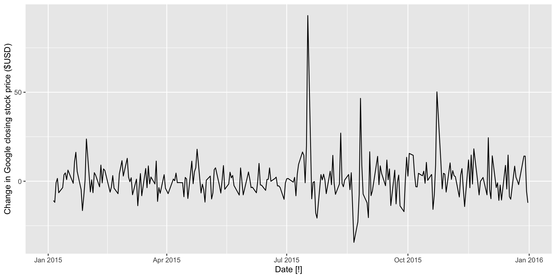
• First difference:

  \[ y_{t}' = y_{t} - y_{t-1} \]

Random walk model

• White noise first difference: \(y_{t}' = \epsilon_{t}\)
• \(y_{t}\) modeled as a random walk:

  \[ y_{t} = y_{t-1} + \epsilon_{t} \]

Example

• Random walk models used for non-stationary data.
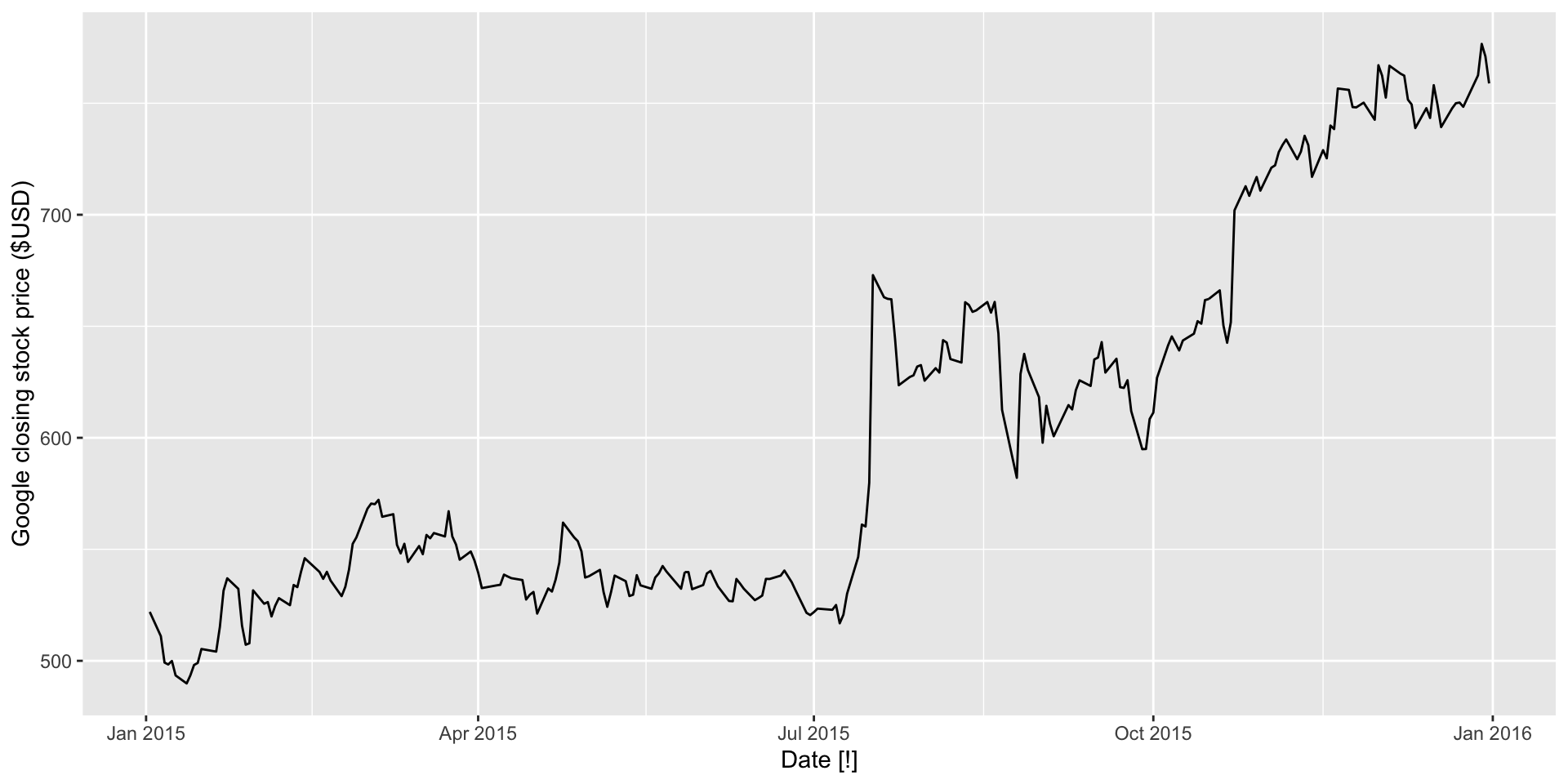
• e.g. Financial data:

google_2015 <- gafa_stock |>
  filter(Symbol == "GOOG", year(Date) == 2015)

Example: plot

Example: first difference plot

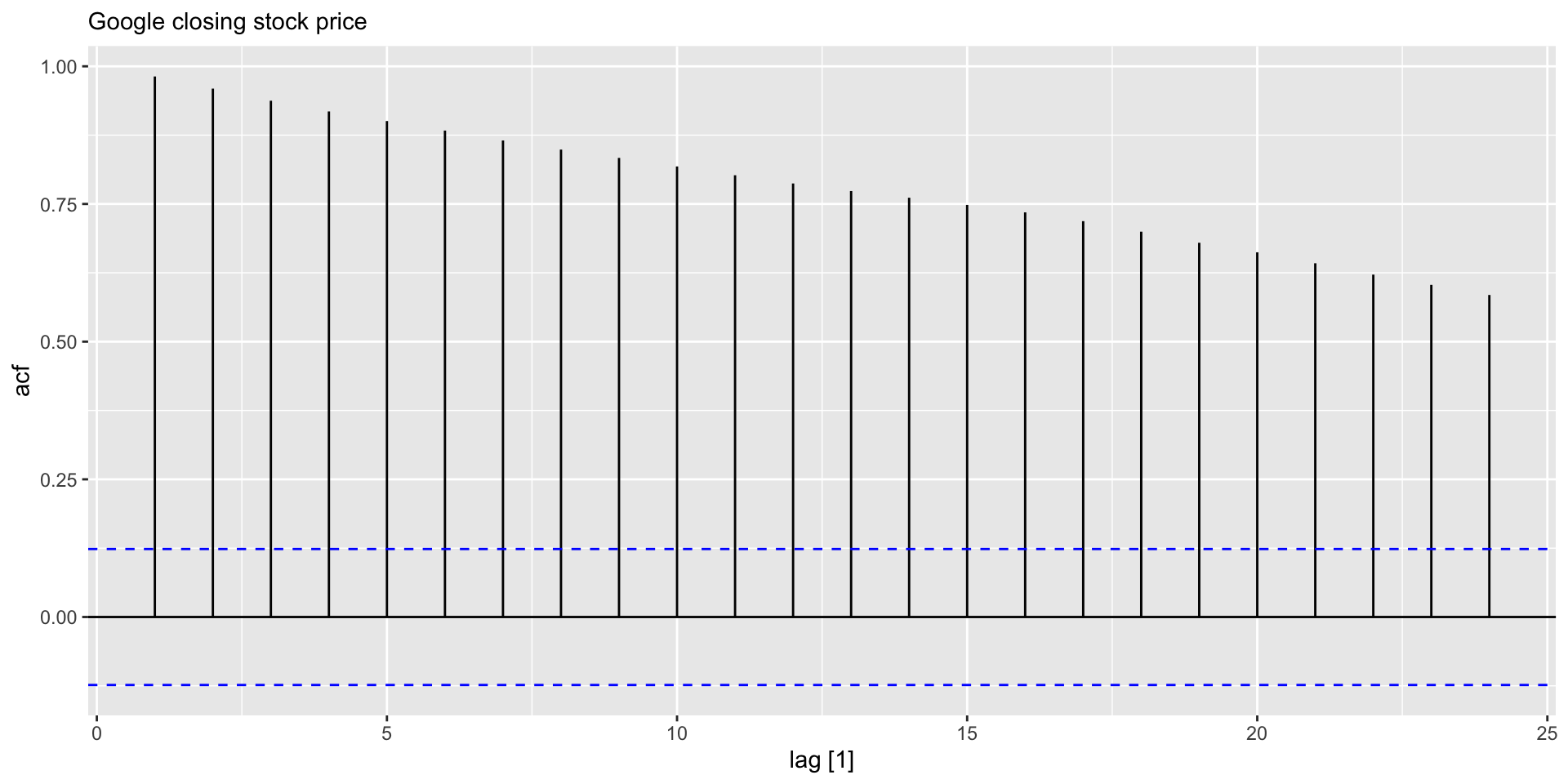
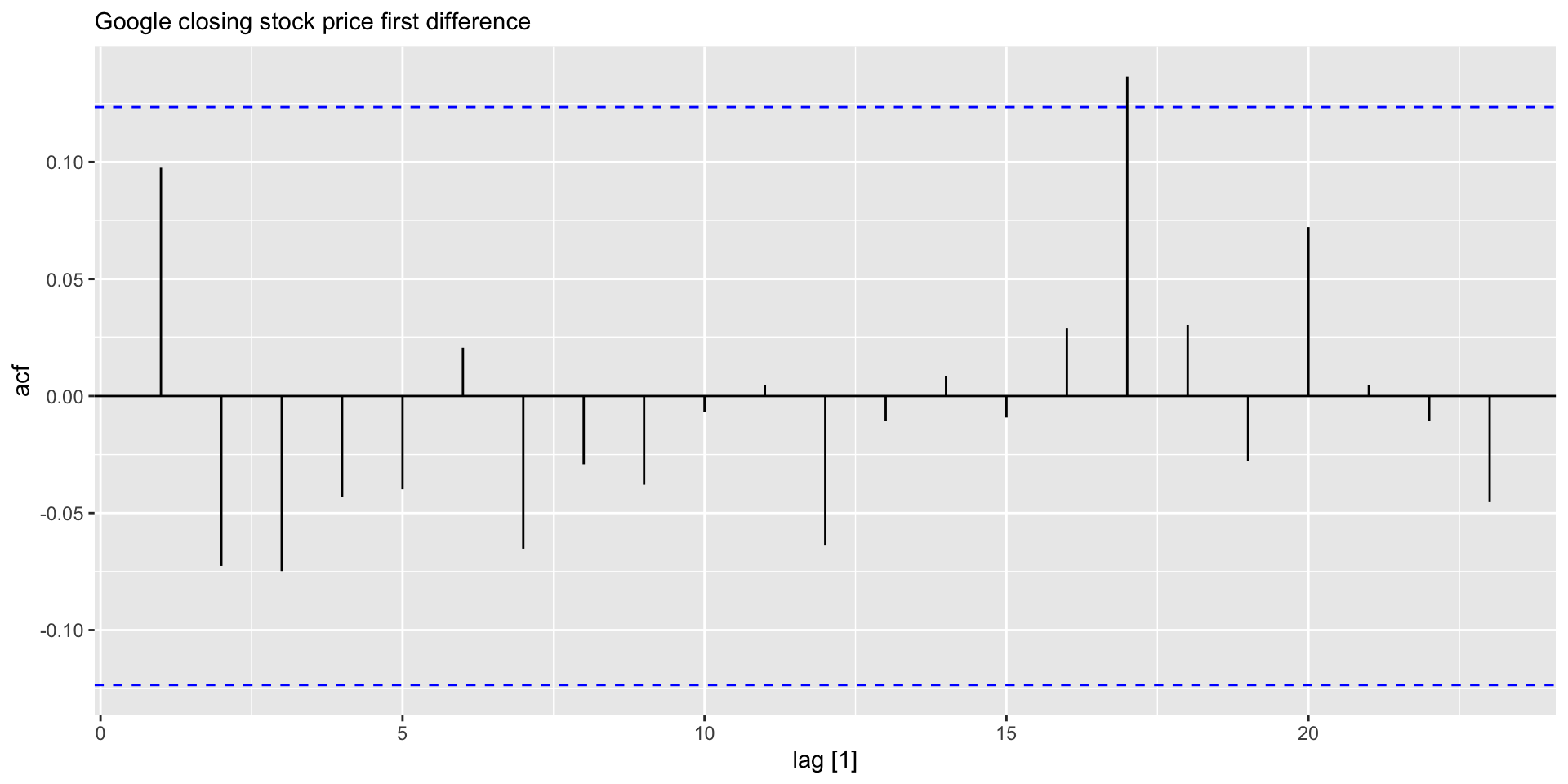
Example: ACF plots

• Check ACF for Google stock price and its first difference:

google_2015 |> ACF(Close) |>
  autoplot() + labs(subtitle = "Google closing stock price")

Example: ACF plots

google_2015 |> ACF(difference(Close)) |>
  autoplot() + labs(subtitle = "Google closing stock price first difference")

Random walk models

• Typical features:
  • Long periods of apparent trends
  • Sudden changes in trend direction
• Random walk model similar to naive model
• Non-zero mean: \(y_{t} = c + y_{t-1} + \epsilon_{t}\) where \(c\) is the average of the changes between consecutive observations.
  • Drift method!

Second differencing

\[ \begin{align} y_{t}'' & = y_{t}' - y_{t-1}' \\ & = (y_{t} - y_{t-1}) - (y_{t-1} - y_{t-2}) \\ & = y_{t} - 2y_{t-1} + y_{t-2} \end{align} \]

• “changes in changes”

Seasonal differencing

\[ y_{t}' = y_{t} - y_{t-m} \]

• “lag-\(m\) differences”
• Yields seasonal naive forecasts.

Implementation

• To take differences easily, use difference()
• To specify \(m\)-step differences, use difference(object, m)