Exponential smoothing

BUS 323 Forecasting and Risk Analysis

Exponential smoothing

Simple model:

\[ \begin{align} \widehat{y}_{T+1|T} = & \alpha y_{T} + \alpha(1-\alpha) y_{T-1} \\ & + \alpha(1-\alpha)^{2} y_{T-2} + ... \end{align} \]
Simple model with trend:

\[ \begin{align} \widehat{y}_{t+h|t} & = l_{t} + hb_{t} \\ l_{t} & = \alpha y_{t} + (1-\alpha)(l_{t-1} + b_{t-1}) \\ b_{t} & = \beta^{*} (l_{t} - l_{t-1}) + (1-\beta^{*})b_{t-1} \end{align} \]
Now we’ll add seasonality.

Holt-Winters’ additive method

Forecast equation:

\[ \widehat{y}_{t+h|t} = l_{t} + hb_{t} + s_{t+h-m(k+1)} \]

\[ \begin{align} l_{t} & = \alpha (y_{t} - s_{t-m}) + (1 - \alpha) (l_{t-1} + b_{t-1}) \\ b_{t} & = \beta^{*} (l_{t} - l_{t-1}) + (1 - \beta^{*}) b_{t-1} \\ s_{t} & = \gamma (y_{t} - l_{t-1} - b_{t-1}) + (1 - \gamma) s_{t-m} \end{align} \]

Holt-Winters’ multiplicative method

\[ \begin{align} \widehat{y}_{t+h|t} & = (l_{t} + h b_{t}) s_{t+h-m(k+1)} \\ l_{t} & = \alpha \frac{y_{t}}{s_{t-m}} + (1 - \alpha) (l_{t-1} + b_{t-1}) \\ b_{t} & = \beta^{*} (l_{t} - l_{t-1}) + (1 - \beta^{*})b_{t-1} \\ s_{t} & = \gamma \frac{y_{t}}{(l_{t-1} + b_{t-1})} + (1 - \gamma) s_{t-m} \end{align} \]

Example: Domestic overnight trips

Let’s examine a data series with a clear seasonal component.
Using the tourism dataset, look at total holiday trips

library(fpp3)
tourism

# A tsibble: 24,320 x 5 [1Q]
# Key:       Region, State, Purpose [304]
   Quarter Region   State           Purpose  Trips
     <qtr> <chr>    <chr>           <chr>    <dbl>
 1 1998 Q1 Adelaide South Australia Business  135.
 2 1998 Q2 Adelaide South Australia Business  110.
 3 1998 Q3 Adelaide South Australia Business  166.
 4 1998 Q4 Adelaide South Australia Business  127.
 5 1999 Q1 Adelaide South Australia Business  137.
 6 1999 Q2 Adelaide South Australia Business  200.
 7 1999 Q3 Adelaide South Australia Business  169.
 8 1999 Q4 Adelaide South Australia Business  134.
 9 2000 Q1 Adelaide South Australia Business  154.
10 2000 Q2 Adelaide South Australia Business  169.
# ℹ 24,310 more rows

Example: Domestic overnight trips

Let’s examine a data series with a clear seasonal component.
Using the tourism dataset, look at total holiday trips
- So we’ll need to filter by Purpose

tourism |>
  filter(Purpose == "Holiday")

# A tsibble: 6,080 x 5 [1Q]
# Key:       Region, State, Purpose [76]
   Quarter Region   State           Purpose Trips
     <qtr> <chr>    <chr>           <chr>   <dbl>
 1 1998 Q1 Adelaide South Australia Holiday  224.
 2 1998 Q2 Adelaide South Australia Holiday  130.
 3 1998 Q3 Adelaide South Australia Holiday  156.
 4 1998 Q4 Adelaide South Australia Holiday  182.
 5 1999 Q1 Adelaide South Australia Holiday  185.
 6 1999 Q2 Adelaide South Australia Holiday  135.
 7 1999 Q3 Adelaide South Australia Holiday  136.
 8 1999 Q4 Adelaide South Australia Holiday  169.
 9 2000 Q1 Adelaide South Australia Holiday  184.
10 2000 Q2 Adelaide South Australia Holiday  134.
# ℹ 6,070 more rows

Example: Domestic overnight trips

Let’s examine a data series with a clear seasonal component.
Using the tourism dataset, look at total holiday trips
- So we’ll need to filter by Purpose
- And sum over all regions.

tourism |>
  filter(Purpose == "Holiday") |>
  summarise(Trips = sum(Trips)/1e3)

# A tsibble: 80 x 2 [1Q]
   Quarter Trips
     <qtr> <dbl>
 1 1998 Q1 11.8 
 2 1998 Q2  9.28
 3 1998 Q3  8.64
 4 1998 Q4  9.30
 5 1999 Q1 11.2 
 6 1999 Q2  9.61
 7 1999 Q3  8.91
 8 1999 Q4  9.03
 9 2000 Q1 11.1 
10 2000 Q2  9.20
# ℹ 70 more rows

Example: Domestic overnight trips

Let’s examine a data series with a clear seasonal component.
Using the tourism dataset, look at total holiday trips
- So we’ll need to filter by Purpose
- And sum over all regions.
- Call the resulting dataset aus_holidays

aus_holidays <- tourism |>
  filter(Purpose == "Holiday") |>
  summarise(Trips = sum(Trips)/1e3)

Example: Domestic overnight trips

To apply the Holt-Winters method, use model(ETS()) as before
- Specify the option season("A") for additive
- season("M") for multiplicative

fit <- aus_holidays |>
  model(
    additive = ETS(Trips ~ error("A") + trend("A") +
                                                season("A")),
    multiplicative = ETS(Trips ~ error("M") + trend("A") +
                                                season("M"))
  )

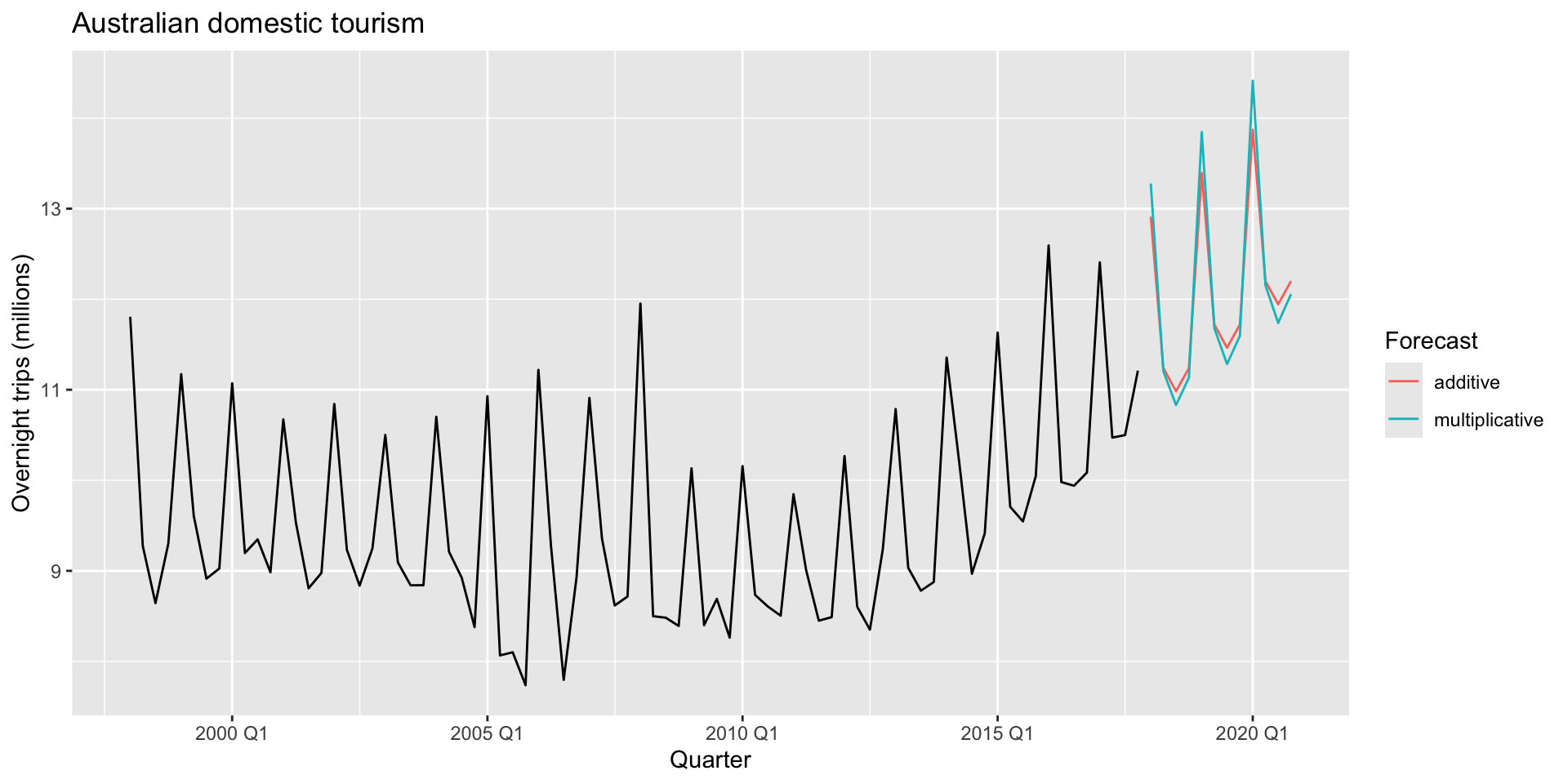
Example: Domestic overnight trips

Produce forecasts for the next three years and plot

fc <- fit |> forecast(h = "3 years")
fc |>
  autoplot(aus_holidays, level = NULL) +
  labs(title="Australian domestic tourism",
       y="Overnight trips (millions)") +
  guides(colour = guide_legend(title = "Forecast"))

Example: Domestic overnight trips

State space models

Each of the models we’ve looked at has:
- A measurement equation that describes observed data
- State equation(s) that describe unobserved components
Taken together, the models are called state space models

State space models

Can be additive or multiplicative
These are broadly referred to as ETS models (Error, Trend, Seasonal)
- Error = A, M
- Trend = N, A, \(A_{d}\)
- Seasonal = N, A, M

ETS(A,N,N)

Recall:

\[ \begin{align} \widehat{y}_{t+1|t} & = l_{t} \\ l_{t} & = \alpha y_{t} + (1 - \alpha) l_{t-1} \end{align} \]

We can re-express the smoothign equation as:

\[ \begin{align} l_{t} & = l_{t-1} + \alpha (y_{t} - l_{t-1}) \\ & = l_{t-1} + \alpha e_{t} \end{align} \]

ETS(A,N,N)

To finally specify our state space model, we have to make an assumption about the probability distribution of the residuals \(e_{t}\).
- With additive errors, residuals are usually assumed \(\epsilon_{t} \sim N(0,\sigma ^{2})\).
Then we can write our model:

\[ \begin{align} \textrm{Measurement equation: } y_{t} & = l_{t-1} + \epsilon_{t} \\ \textrm{State equation: } l_{t} & = l_{t-1} + \alpha \epsilon_{t} \end{align} \]

A taxonomy of ETS models

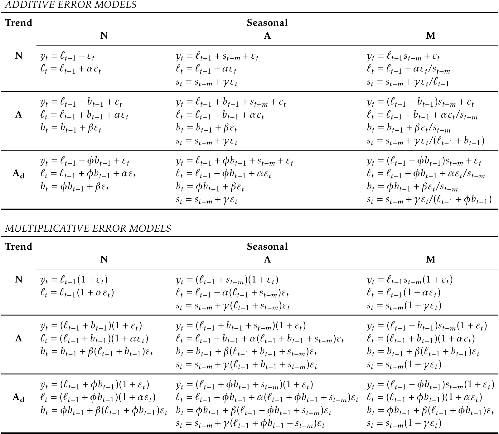
Figure: Measurement and state equations for various ETS models