Evaluating forecast accuracy

BUS 323 Forecasting and Risk Analysis

Training and test sets

Accuracy: more than error size
- Evaluate forecast performance on historical data
- Separate into training and test sets
  - Test set: ~20% of the full sample
  - Or at least as large as the forecast horizon

Training and test sets

A couple things to note:
- Good fit with training data \(\neq\) good forecast
- More parameters \(\rightarrow\) perfect fit
- Over-fitting does not yield a good forecast.
“Test set” aka “holdout set” or “out-of-sample data”.

Subsetting functions

filter()
- e.g. To extract all data from 1995 onward:

library(fpp3)
aus_production |> filter(year(Quarter) >= 1995)

# A tsibble: 62 x 7 [1Q]
   Quarter  Beer Tobacco Bricks Cement Electricity   Gas
     <qtr> <dbl>   <dbl>  <dbl>  <dbl>       <dbl> <dbl>
 1 1995 Q1   426    4714    430   1626       41768   131
 2 1995 Q2   408    3939    457   1703       43686   167
 3 1995 Q3   416    6137    417   1733       46022   181
 4 1995 Q4   520    4739    370   1545       42800   145
 5 1996 Q1   409    4275    310   1526       43661   133
 6 1996 Q2   398    5239    358   1593       44707   162
 7 1996 Q3   398    6293    379   1706       46326   184
 8 1996 Q4   507    5575    369   1699       43346   146
 9 1997 Q1   432    4802    330   1511       43938   135
10 1997 Q2   398    5523    390   1785       45828   171
# ℹ 52 more rows

Subsetting functions

filter()
- Equivalently:

aus_production |> filter_index("1995 Q1" ~ .)

# A tsibble: 62 x 7 [1Q]
   Quarter  Beer Tobacco Bricks Cement Electricity   Gas
     <qtr> <dbl>   <dbl>  <dbl>  <dbl>       <dbl> <dbl>
 1 1995 Q1   426    4714    430   1626       41768   131
 2 1995 Q2   408    3939    457   1703       43686   167
 3 1995 Q3   416    6137    417   1733       46022   181
 4 1995 Q4   520    4739    370   1545       42800   145
 5 1996 Q1   409    4275    310   1526       43661   133
 6 1996 Q2   398    5239    358   1593       44707   162
 7 1996 Q3   398    6293    379   1706       46326   184
 8 1996 Q4   507    5575    369   1699       43346   146
 9 1997 Q1   432    4802    330   1511       43938   135
10 1997 Q2   398    5523    390   1785       45828   171
# ℹ 52 more rows

Subsetting functions

slice()
- To extract the last 20 observations:

aus_production |>
  slice(n()-19:0)

# A tsibble: 20 x 7 [1Q]
   Quarter  Beer Tobacco Bricks Cement Electricity   Gas
     <qtr> <dbl>   <dbl>  <dbl>  <dbl>       <dbl> <dbl>
 1 2005 Q3   408      NA     NA   2340       56043   221
 2 2005 Q4   482      NA     NA   2265       54992   180
 3 2006 Q1   438      NA     NA   2027       57112   171
 4 2006 Q2   386      NA     NA   2278       57157   224
 5 2006 Q3   405      NA     NA   2427       58400   233
 6 2006 Q4   491      NA     NA   2451       56249   192
 7 2007 Q1   427      NA     NA   2140       56244   187
 8 2007 Q2   383      NA     NA   2362       55036   234
 9 2007 Q3   394      NA     NA   2536       59806   245
10 2007 Q4   473      NA     NA   2562       56411   205
11 2008 Q1   420      NA     NA   2183       59118   194
12 2008 Q2   390      NA     NA   2558       56660   229
13 2008 Q3   410      NA     NA   2612       64067   249
14 2008 Q4   488      NA     NA   2373       59045   203
15 2009 Q1   415      NA     NA   1963       58368   196
16 2009 Q2   398      NA     NA   2160       57471   238
17 2009 Q3   419      NA     NA   2325       58394   252
18 2009 Q4   488      NA     NA   2273       57336   210
19 2010 Q1   414      NA     NA   1904       58309   205
20 2010 Q2   374      NA     NA   2401       58041   236

Subsetting functions

slice()
- To subset the first year of data from each State and Industry:

aus_retail |>
  group_by(State, Industry) |>
  slice(1:12)

# A tsibble: 1,824 x 5 [1M]
# Key:       State, Industry [152]
# Groups:    State, Industry [152]
   State                        Industry           `Series ID`    Month Turnover
   <chr>                        <chr>              <chr>          <mth>    <dbl>
 1 Australian Capital Territory Cafes, restaurant… A3349849A   1982 Apr      4.4
 2 Australian Capital Territory Cafes, restaurant… A3349849A   1982 May      3.4
 3 Australian Capital Territory Cafes, restaurant… A3349849A   1982 Jun      3.6
 4 Australian Capital Territory Cafes, restaurant… A3349849A   1982 Jul      4  
 5 Australian Capital Territory Cafes, restaurant… A3349849A   1982 Aug      3.6
 6 Australian Capital Territory Cafes, restaurant… A3349849A   1982 Sep      4.2
 7 Australian Capital Territory Cafes, restaurant… A3349849A   1982 Oct      4.8
 8 Australian Capital Territory Cafes, restaurant… A3349849A   1982 Nov      5.4
 9 Australian Capital Territory Cafes, restaurant… A3349849A   1982 Dec      6.9
10 Australian Capital Territory Cafes, restaurant… A3349849A   1983 Jan      3.8
# ℹ 1,814 more rows

Forecast errors

Forecast residuals based on training set.
Forecast errors based on test set.

\[ e_{T+h} = y_{T+h} - \widehat{y}_{T+h|T} \]
- We’ll use these to evaluate forecast accuracy.

Scale-dependent errors

Forecast errors are on the same scale as the time series being forecasted.
- Any measure of accuracy based on errors will be similarly scaled.
Two common measures:

\[ \textrm{Mean absolute error: } MAE = \bar{|e_{t}|} \]

\[ \textrm{Root mean squared error: } RMSE = \sqrt{\bar{e_{t}}^{2}} \]
- RMSE commonly used as an objective function for forecast methods.

Percentage errors

Used to compare performance across time series
Most common measure:

\[ \textrm{Mean absolute percentage error: } MAPE = \bar{|p_{t}|} \]
- Where \(p_{t} = 100 \frac{e_{t}}{y_{t}}\).
Percentage errors cause problems when \(y_{t}\) is small.

Example: defining train/test

Use aus_production. Filter such that year is \(\geq\) 1992. Then define the period 1992-2007 as the training set:

recent_production <- aus_production |>
  filter(year(Quarter) >= 1992)
beer_train <- recent_production |>
  filter(year(Quarter) <= 2007)

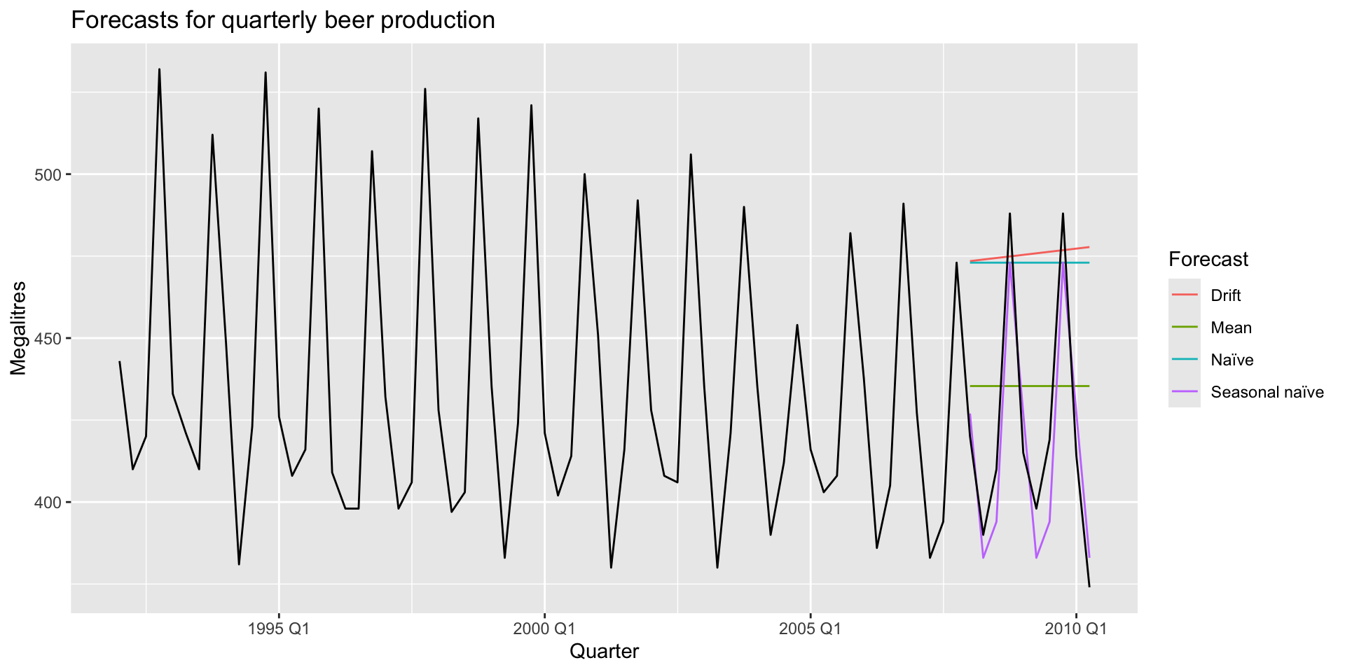
Example: forecasting

10 observations exist in the test set. Produce a mean, naive, seasonal naive, and drift forecast for those observations.

beer_fit <- beer_train |>
  model(
    Mean = MEAN(Beer),
    `Naïve` = NAIVE(Beer),
    `Seasonal naïve` = SNAIVE(Beer),
    Drift = RW(Beer ~ drift())
  )

beer_fc <- beer_fit |>
  forecast(h = 10)

Example: plotting

Plot all forecasts with autoplot() and add in observed data:

beer_fc |>
  autoplot(
    aus_production |> filter(year(Quarter) >= 1992),
    level = NULL
  ) +
  labs(
    y = "Megalitres",
    title = "Forecasts for quarterly beer production"
  ) +
  guides(colour = guide_legend(title = "Forecast"))

Example: plotting

Example: forecast accuracy

Use the accuracy() function. Supply the forecast object (beer_fc) and the observed data (`recent_production)

accuracy(beer_fc, recent_production)

# A tibble: 4 × 10
  .model         .type    ME  RMSE   MAE    MPE  MAPE  MASE RMSSE    ACF1
  <chr>          <chr> <dbl> <dbl> <dbl>  <dbl> <dbl> <dbl> <dbl>   <dbl>
1 Drift          Test  -54.0  64.9  58.9 -13.6  14.6  4.12  3.87  -0.0741
2 Mean           Test  -13.8  38.4  34.8  -3.97  8.28 2.44  2.29  -0.0691
3 Naïve          Test  -51.4  62.7  57.4 -13.0  14.2  4.01  3.74  -0.0691
4 Seasonal naïve Test    5.2  14.3  13.4   1.15  3.17 0.937 0.853  0.132

Example: Google stock price

Use the 2015 Google stock price data previously constructed. We’ll produce forecasts for January 2016.

# Re-index based on trading days
google_stock <- gafa_stock |>
  filter(Symbol == "GOOG", year(Date) >= 2015) |>
  mutate(day = row_number()) |>
  update_tsibble(index = day, regular = TRUE)
# Filter for training set
google_2015 <- google_stock |> filter(year(Date) == 2015)
# Filter for test set
google_jan_2016 <- google_stock |>
  filter(yearmonth(Date) == yearmonth("2016 Jan"))

Example: Google stock price

Produce a mean, naive, and drift forecast for January 2016. Plot the historical data and the forecasts.

google_fit <- google_2015 |>
  model(
    Mean = MEAN(Close),
    `Naïve` = NAIVE(Close),
    Drift = RW(Close ~ drift())
  )

google_fc <- google_fit |>
  forecast(google_jan_2016)

Example: Google stock price

Evaluate each forecast’s accuracy.

accuracy(google_fc, google_stock)

# A tibble: 3 × 11
  .model Symbol .type    ME  RMSE   MAE   MPE  MAPE  MASE RMSSE  ACF1
  <chr>  <chr>  <chr> <dbl> <dbl> <dbl> <dbl> <dbl> <dbl> <dbl> <dbl>
1 Drift  GOOG   Test  -49.8  53.1  49.8 -6.99  6.99  6.99  4.74 0.604
2 Mean   GOOG   Test  117.  118.  117.  16.2  16.2  16.4  10.5  0.496
3 Naïve  GOOG   Test  -40.4  43.4  40.4 -5.67  5.67  5.67  3.88 0.496