Forecasting with transformations and decomposition

BUS 323 Forecasting and Risk Analysis

Forecasting with transformed data

Tranform data to improve forecast stability \(w_{t} = f(y_{t}\))
- Forecast transformed variable \(w_{t}\)
- Back-transform to obtain forecasts for \(y_{t}\)

Prediction intervals with transformed data

Prediction interval computed for \(\widehat{w}_{t}\)
- End-points back-transformed
- Prediction interval not necessarily symmetric

Bias adjustments

Back-transformed point forecast not necessarily mean
- Typically median
- Problem?
- Larger variance \(\rightarrow\) more difference between median and mean

Example: Box-Cox transformation

The back-transformation for a Box-Cox transformation is given by:

\[ \widehat{y}_{T+h|T} = \left\{\begin{array}{lr} exp(\widehat{w}_{T+h|T}) & \textrm{if} \lambda=0; \\ sin(\lambda \widehat{w}_{T+h|T} + 1)(\lambda \widehat{w}_{T+h|T} + 1)^{1/\lambda} & \textrm{otherwise}. \end{array}\right\} \]
This returns the median of the prediction interval.

Example: Box-Cox transformation

The back-tranformed mean is given by:
\[ \widehat{y}_{T+h|T} = \left\{\begin{array}{lr} exp(\widehat{w}_{T+h|T})[1 + \frac{\sigma_{h}^{2}}{2}] & \textrm{if} \lambda=0; \\ (\lambda \widehat{w}_{T+h|T} + 1)^{1/\lambda}[1 + \frac{\sigma_{h}^{2}(1-\lambda)}{2(\lambda \widehat{w}_{T+h|T} + 1)^{2}}] & \textrm{otherwise} \end{array}\right\} \] where \(\widehat{w}_{T+h|T}\) is the \(h\)-step forecast mean and \(\sigma_{h}^{2}\) is the \(h\)-step forecast variance on the transformed scale.

Bias adjustments

bias: The difference between the back-transformed forecast and the mean forecast
bias-adjusted: uses the mean forecast rather than the back-transformed forecast

Bias adjustments: example

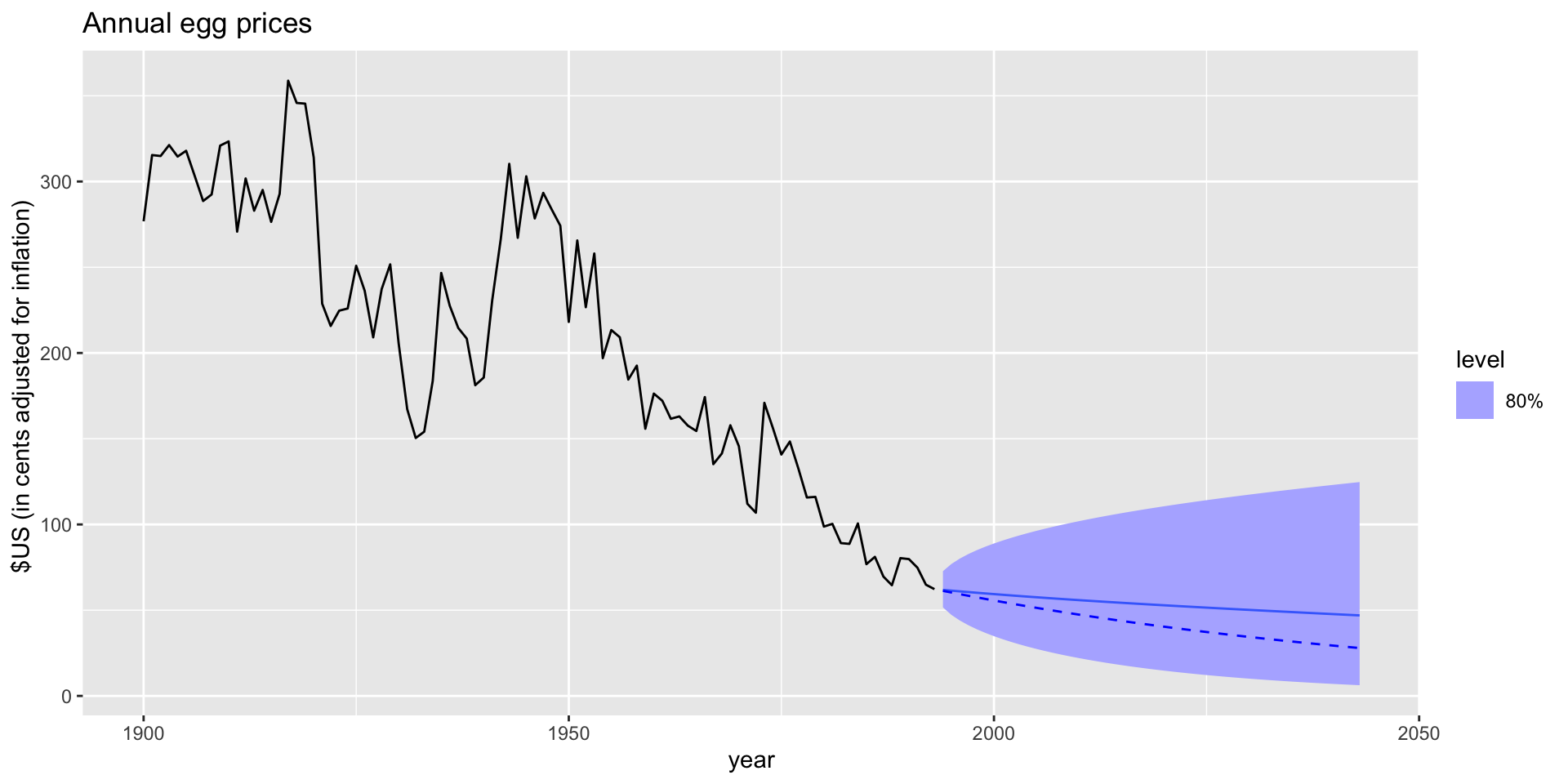
Drift forecast of egg prices using a log transformation.

Solid line: mean; dashed line: median

Bias adjustments: example

Back-transformed means automatically calculated with fable.
- Median accessible using median() on the distribution variable.

prices |>
  filter(!is.na(eggs))

# A tsibble: 94 x 7 [1Y]
    year  eggs chicken copper nails   oil wheat
   <dbl> <dbl>   <dbl>  <dbl> <dbl> <dbl> <dbl>
 1  1900  277.      NA   6.81  54.1  23.1  399.
 2  1901  315.      NA   6.94  48.6  18.6  404.
 3  1902  315.      NA   4.74  41.6  14.9  425.
 4  1903  321.      NA   5.21  39.5  16.9  399.
 5  1904  315.      NA   4.98  36.3  15.5  416.
 6  1905  318.      NA   6.01  36.1  11.2  437.
 7  1906  303.      NA   7.45  37.3  13.1  410.
 8  1907  289.      NA   7.81  38.9  12.5  439.
 9  1908  292.      NA   5.18  40.0  13.0  469.
10  1909  321.      NA   5.10  36.5  12.6  531.
# ℹ 84 more rows

Bias adjustments: example

prices |>
  filter(!is.na(eggs)) |>
    model(RW(log(eggs) ~ drift()))

# A mable: 1 x 1
  `RW(log(eggs) ~ drift())`
                    <model>
1             <RW w/ drift>

Bias adjustments: example

prices |>
  filter(!is.na(eggs)) |>
    model(RW(log(eggs) ~ drift())) |>
      forecast(h = 50)

# A fable: 50 x 4 [1Y]
# Key:     .model [1]
   .model                   year             eggs .mean
   <chr>                   <dbl>           <dist> <dbl>
 1 RW(log(eggs) ~ drift())  1994 t(N(4.1, 0.018))  61.8
 2 RW(log(eggs) ~ drift())  1995 t(N(4.1, 0.036))  61.4
 3 RW(log(eggs) ~ drift())  1996 t(N(4.1, 0.055))  61.0
 4 RW(log(eggs) ~ drift())  1997 t(N(4.1, 0.074))  60.6
 5 RW(log(eggs) ~ drift())  1998 t(N(4.1, 0.093))  60.2
 6 RW(log(eggs) ~ drift())  1999    t(N(4, 0.11))  59.8
 7 RW(log(eggs) ~ drift())  2000    t(N(4, 0.13))  59.4
 8 RW(log(eggs) ~ drift())  2001    t(N(4, 0.15))  59.0
 9 RW(log(eggs) ~ drift())  2002    t(N(4, 0.18))  58.6
10 RW(log(eggs) ~ drift())  2003     t(N(4, 0.2))  58.3
# ℹ 40 more rows

Bias adjustments: example

prices |>
  filter(!is.na(eggs)) |>
    model(RW(log(eggs) ~ drift())) |>
      forecast(h = 50) |>
        mutate(.median = median(eggs))

# A fable: 50 x 5 [1Y]
# Key:     .model [1]
   .model                   year             eggs .mean .median
   <chr>                   <dbl>           <dist> <dbl>   <dbl>
 1 RW(log(eggs) ~ drift())  1994 t(N(4.1, 0.018))  61.8    61.3
 2 RW(log(eggs) ~ drift())  1995 t(N(4.1, 0.036))  61.4    60.3
 3 RW(log(eggs) ~ drift())  1996 t(N(4.1, 0.055))  61.0    59.3
 4 RW(log(eggs) ~ drift())  1997 t(N(4.1, 0.074))  60.6    58.4
 5 RW(log(eggs) ~ drift())  1998 t(N(4.1, 0.093))  60.2    57.5
 6 RW(log(eggs) ~ drift())  1999    t(N(4, 0.11))  59.8    56.6
 7 RW(log(eggs) ~ drift())  2000    t(N(4, 0.13))  59.4    55.7
 8 RW(log(eggs) ~ drift())  2001    t(N(4, 0.15))  59.0    54.8
 9 RW(log(eggs) ~ drift())  2002    t(N(4, 0.18))  58.6    53.9
10 RW(log(eggs) ~ drift())  2003     t(N(4, 0.2))  58.3    53.0
# ℹ 40 more rows

Recall: decomposed vaiables

Additive: \(y_{t} = \widehat{S}_{t} + \widehat{A}_{t}\)
- where \(\widehat{A}_{t} = \widehat{T}_{t} + \widehat{R}_{t}\) is the seasonally adjusted component.
Multiplicative: \(y_{t} = \widehat{S}_{t}\widehat{A}_{t}\)

Forecasting with decomposed variables

To forecast, forecast \(\widehat{S}_{t}\) and \(\widehat{A}_{t}\) separately.
- \(\widehat{S}_{t}\) typically assumed unchanging
  - Thus a seasonal naive method used for \(\widehat{S}_{t}\)
- \(\widehat{A}_{t}\) can be forecasted with any appropriate method.

Example: US retail employment

First, filter us_retail_employment to year>=1990 and Title=="Retail Trade"

us_retail_employment <- us_employment |>
  filter(year(Month) >= 1990, Title == "Retail Trade")

Example: US retail employment

Next, use an STL decompositionL

dcmp <- us_retail_employment |>
  model(STL(Employed ~ trend(window = 7), robust = TRUE))

Example: US retail employment

Let’s look at the components:

dcmp <- us_retail_employment |>
  model(STL(Employed ~ trend(window = 7), robust = TRUE)) |>
  components()
dcmp

# A dable: 357 x 8 [1M]
# Key:     Series_ID, .model [1]
# :        Employed = trend + season_year + remainder
   Series_ID .model    Month Employed  trend season_year remainder season_adjust
   <chr>     <chr>     <mth>    <dbl>  <dbl>       <dbl>     <dbl>         <dbl>
 1 CEU42000… STL(E… 1990 Jan   13256. 13326.       -72.6     2.85         13328.
 2 CEU42000… STL(E… 1990 Feb   12966. 13297.      -273.    -58.1          13239.
 3 CEU42000… STL(E… 1990 Mar   12938. 13270.      -295.    -36.3          13233.
 4 CEU42000… STL(E… 1990 Apr   13012. 13230.      -216.     -1.59         13228.
 5 CEU42000… STL(E… 1990 May   13108. 13223.      -119.      4.72         13228.
 6 CEU42000… STL(E… 1990 Jun   13183. 13212.       -30.6     0.978        13213.
 7 CEU42000… STL(E… 1990 Jul   13170. 13198.       -32.8     5.23         13203.
 8 CEU42000… STL(E… 1990 Aug   13160. 13178.       -20.1     1.84         13180.
 9 CEU42000… STL(E… 1990 Sep   13113. 13149.       -45.5     9.76         13159.
10 CEU42000… STL(E… 1990 Oct   13185. 13113.        64.2     8.28         13121.
# ℹ 347 more rows

Example: US retail employment

And remove the .model column:

us_retail_employment <- us_employment |>
  filter(year(Month) >= 1990, Title == "Retail Trade")
dcmp <- us_retail_employment |>
  model(STL(Employed ~ trend(window = 7), robust = TRUE)) |>
  components() |>
  select(-.model)

Example: US retail employment

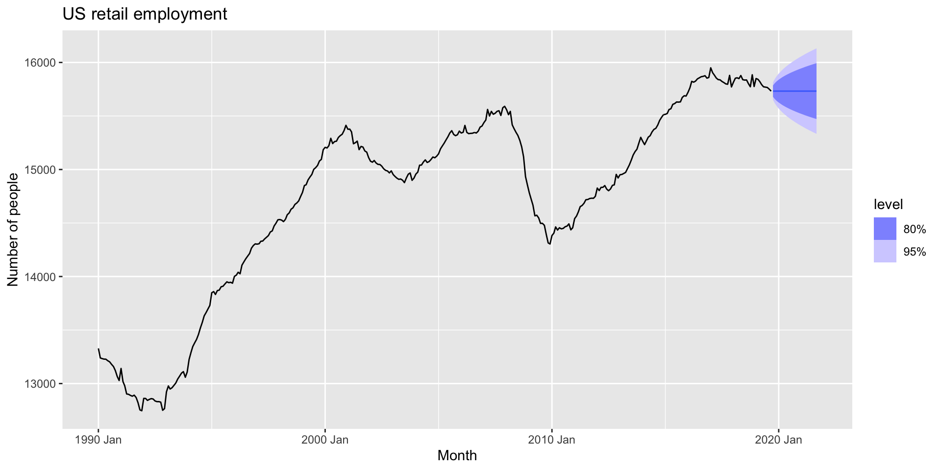
Next, make a naive forecast the seasonally adjusted component:

dcmp |>
  model(NAIVE(season_adjust)) |>
  forecast()

# A fable: 24 x 5 [1M]
# Key:     Series_ID, .model [1]
   Series_ID     .model                  Month
   <chr>         <chr>                   <mth>
 1 CEU4200000001 NAIVE(season_adjust) 2019 Oct
 2 CEU4200000001 NAIVE(season_adjust) 2019 Nov
 3 CEU4200000001 NAIVE(season_adjust) 2019 Dec
 4 CEU4200000001 NAIVE(season_adjust) 2020 Jan
 5 CEU4200000001 NAIVE(season_adjust) 2020 Feb
 6 CEU4200000001 NAIVE(season_adjust) 2020 Mar
 7 CEU4200000001 NAIVE(season_adjust) 2020 Apr
 8 CEU4200000001 NAIVE(season_adjust) 2020 May
 9 CEU4200000001 NAIVE(season_adjust) 2020 Jun
10 CEU4200000001 NAIVE(season_adjust) 2020 Jul
# ℹ 14 more rows
# ℹ 2 more variables: season_adjust <dist>, .mean <dbl>

Example: US retail employment

Finally, use autoplot() to plot the forecast with the seasonal component added back in:

dcmp |>
  model(NAIVE(season_adjust)) |>
  forecast() |>
  autoplot(dcmp) +
  labs(y = "Number of people",
       title = "US retail employment")

Example: US retail employment

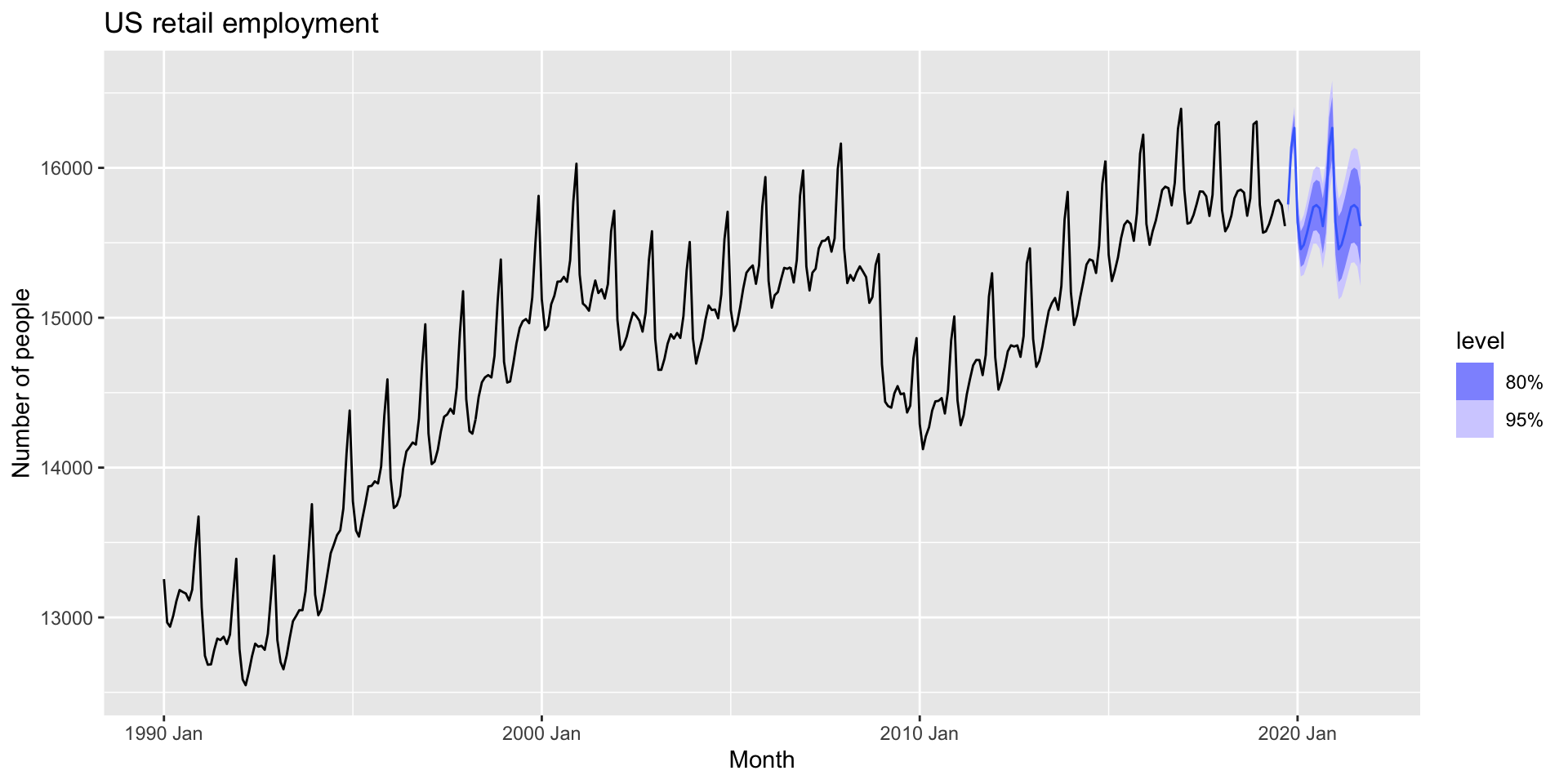
`decomposition_model()`

The decomposition_model() function makes this a bit simpler.
- Seasonal naive forecasts are used for the seasonal component automatically.
- Also reseasonalizes the forecasts for you for observed data:

fit_dcmp <- us_retail_employment |>
  model(stlf = decomposition_model(
    STL(Employed ~ trend(window = 7), robust = TRUE),
    NAIVE(season_adjust)
  ))

`decomposition_model()` forecasts

autoplot() will plot the forecasts for the original data as well as future forecasts:

fit_dcmp |>
  forecast() |>
  autoplot(us_retail_employment)+
  labs(y = "Number of people",
       title = "US retail employment")

Forecasting with transformations and decomposition

Forecasting with transformed data

Prediction intervals with transformed data

Bias adjustments

Example: Box-Cox transformation

Example: Box-Cox transformation

Bias adjustments

Bias adjustments: example

Bias adjustments: example

Bias adjustments: example

Bias adjustments: example

Bias adjustments: example

Recall: decomposed vaiables

Forecasting with decomposed variables

Example: US retail employment

Example: US retail employment

Example: US retail employment

Example: US retail employment

Example: US retail employment

Example: US retail employment

Example: US retail employment

decomposition_model()

decomposition_model() forecasts

decomposition_model() plot

`decomposition_model()`

`decomposition_model()` forecasts

`decomposition_model()` plot